Download
1 / 31
310 likes | 425 Views
S.Frasca on behalf of LSC-Virgo collaboration. The search for Vela pulsar in Virgo VSR1 data. New York, J une 23 rd , 2009. The Vela Pulsar. Right ascension: 8h 35m 20.61149 s Declination: -45º 10’ 34.8751 s Period: ~89.36 ms Distance: 290 pc

E N D
S.Frasca on behalf of LSC-Virgo collaboration The search for Vela pulsar in Virgo VSR1 data New York, June 23rd, 2009
The Vela Pulsar Right ascension: 8h 35m 20.61149 s Declination: -45º 10’ 34.8751 s Period: ~89.36 ms Distance: 290 pc Glitch occurred between day 24 July and 13 August of 2007 Ephemerides supplied by Aidan Hotan and Jim Palfreymanusing the Mt. PleasantRadiotelscope (Hobart, Tasmania) (period 25 Aug – 6 Sept) Spin-down limit: 3.3e-24 Presumed ψ=131º, ι=61º (ε=0.51)
The selected Virgo data are from 13 Aug 2007 6:38 to the end of the run (1 October) Ephemerides, given for the period 25 August – 6 September, wereextrapolated The data used
For a gravitational wave described by where the two κ are real positive constants, we the response of the antenna is with where the constants a and b depend on the position of the source and of the antenna. So the whole information on a signal (and on the noise) is in 5 complex numbers. The source and the antenna
The source and the antenna Energy of the wave that goes into the antenna, for all types of waves from Vela If we describe the wave with an elliptical polarization of semi-axes a and b normalized such that we have (being a ≥ b ) ψ is the polarization angle of the linearly polarized part.
Create the (cleaned) SFT data base (after this step all the analysis is done on a workstation with Matlab) • Extract a 0.25 Hz band • Reconstruct the time signal with the Doppler and spin-down correction • Eliminate bad periods and disturbances • Apply the “Noise Wiener filter” • Simulate four basic signals • Apply the 5 components matched filter • Find the best source for the data • Enlarge the analysis to the near frequencies Scheme of the procedure
Our Short FFTs are computed on the length of 1024 s and interlaced In our period we have about 7000 FFTs Our h data are multiplied by1020 The SFT data base
The data of the SFTs in the band 22.25~22.50 are extracted in a single file of about 15 MB From these we reconstruct a time series with 1 Hz sampling time (and zero where there are holes), correcting for the Doppler effect and the spin-down. We obtain data with “apparent frequency” 22.38194046 Hz. Band extraction and Time data reconstruction
The data are not stationary, so the sensitivity of the antenna is not constant in the observation period. To optimize for this feature we introduced the “Noise Wiener Filter” as where σ2(t) is the slowly varying variance of the data. W(t) multiplies the time data. “Noise Wiener Filter”
Spectrum of the selected data (after the NWF) Full band (1 Hz), selected part and histogram of the Wiener filtered data power spectrum. Spectrum : µ = 2.0063, σ = 2.0070 selected about 2 million spectral data (resolution=2)
The same band extraction function is used to simulate the basic signals from Vela. The same Doppler and spin-down correction, the same cuts and the same Wiener filter, that we applied to the Virgo data, have been applied to the signals data. The simulated signals were the 2 linearly polarized signals and the 2 circularly polarized signals in both left and right rotation. The amplitude was h0=10-20. The Signal and the simulations
As it is well known, the signal contains only the 5 frequencies f0, f0±Fs and f0±2Fs , where f0 is the (apparent) frequency of the signal and Fs is the sidereal frequency. So we can consider only the components of the signal and of the noise at that frequencies, that means 5 complex numbers. For two signal that differ only in phase, these 5 numbers are all multiplied for the same complex coefficient ejφ. The basic idea of the 5-components matched filter is that the best way to detect a signal s (bold means a quintuplet of complex numbers) in a signal+noise combination d = A s + n we do the estimation of the complex number A=A0ejφ as where s’ is the complex conjugate. We obtain the 5-components for any signal from the simulated basic signals, that has been treated exactly as the data. It is convenient to consider the squared value of the estimated A0; in this case, in absence of signal, we have an exponential distribution. The Matched filter
For each evaluation of the matched filter we compute also the squared coherence of the estimated signal with the data as where s and d are the signal and data quintuplets, as in the previous slide. The Coherence
Application of the 4 basic matched filters Squared output of the matched filter applied to the data and to all the signals Coherences for the above filters
Application of the 4 basic matched filters: background Blue: Linear ψ=0 Green: Linear ψ=45 Red: Circular CCW Cyan: Circular CW MeanStdSignal 4.67e-6 4.67e-6 2.78e-6 4.39e-6 4.39e-6 1.064e-5 4.53e-6 4.52e-6 5.15e-6 4.53e-6 4.53e-6 9.08e-6 (the signal is estimated by linear approximation)
Application of the 4 basic matched filters: background Histograms of the squared modulus of the 4 matched filters applied to the sub-band.
Application of the 4 basic matched filters: results for all the signals The maximum is for ε=0.78, ψ=57º, CW ; here the value of the map is about 12.6e-6. This means amplitude 3.6 10-23 . The squared SNR is about 2.8 and Prob=exp(-2.8) ~ 0.061 . So the upper limit is 3.6 10-23 .
Application of the 4 basic matched filters: Coherence for all the signals For the maximum, the coherence is about 0.51 .
The A estimated for each signal by the matched filter can be seen as the component of the data “along that signal”. So if a signal is a linear combination of 2 orthogonal signals (as the + and x or the CCW and CW signals are), we can obtain the output of that signal as the same combination of the matched filter applied to the 2 signals. We can compute the distribution of the squared modulus of the matched filter output of this “maximum” signal and the coherence. The best polarization statistics (F-statistics)
The best polarization statistics (F-statistics) – the background
The best polarization statistics (F-statistics) – The distribution
The best polarization statistics (F-statistics) – the coherence
Browsing around(about 8 million frequencies in 0.24 Hz) Coherence (crosses) with normalized quadratic response of the 4 matched filters
Coherence probability Probability to have a coherence bigger than a certain value.
Browsing around The graph shows the maximum of the normalized absolute square of the 4 basic matched filters applied at frequencies near the apparent frequency. The abscissa is the distance from the apparent frequency.