Network Simulation

1. Motivation: learn fundamentals of evaluating network performance via simulation Overview: fundamentals of discrete event simulation analyzing simulation outputs ns-2 simulation Network Simulation

2. The evaluation spectrum simulation prototype numerical models emulation operational system

3. program boundary computer program simulates deterministic rules governing behavior pseudo random inputs to system (models environment) “simulated” life observer What is simulation? system boundary system under study (has deterministic rules governing its behavior) exogenous inputs to system (the environment) “real” life observer

4. Why Simulation? • goal: study system performance, operation • real-system not available, is complex/costly or dangerous (eg: space simulations, flight simulations) • quickly evaluate design alternatives (eg: different system configurations) • evaluate complex functions for which closed form formulas or numerical techniques not available

5. Simulation: advantages/drawbacks • advantages: • drawbacks/dangers:

6. Programming a simulation What ‘s in a simulation program? • simulated time: internal (to simulation program) variable that keeps track of simulated time • system “state”: variables maintained by simulation program define system “state” • e.g., may track number (possibly order) of packets in queue, current value of retransmission timer • events: points in time when system changes state • each event has associated event time • e.g., arrival of packet to queue, departure from queue • precisely at these points in time that simulation must take action (change state and may cause new future events) • model for time between events (probabilistic) caused by external environment

7. Discrete Event Simulation • simulation program maintains and updates list of future events: event list • simulator structure: initialize event list get next (nearest future) event from event list Need: • well defined set of events • for each event: simulated system action, updating of event list time = event time process event (change state values, add/delete future events from event list update statistics n done? y

8. Simulation: example • packets arrive (avg. interrarrival time: 1/ l) to router (avg. execution time 1/m) with two outgoing links • arriving packet joins link i with probability fi m1 l m2 • state of system: size of each queue • system events: • job arrivals • service time completions • define performance measure to be gathered

9. m1 l m2 Simulation: example Simulator actions on arrival event • choose a link • if link idle {place pkt in service, determine service time (random number drawn from service time distribution) add future event onto event list for pkt transfer completion, set number of pkts in queue to 1} • if buffer full {increment # dropped packets, ignore arrival} • else increment number in queue where queued • create event for next arrival (generate interarrival time) stick event on event list

10. m1 l m2 Simulation: example Simulator actions on departure event • remove event, update simulation time, update performance statistics • decrement counter of number of pkts in queue • If (number of jobs in queue > 0) put next pkt into service – schedule completion event (generate service time for put)

11. total simulated time Gathering Performance Statistics • avg delay at queue i: record Dij : delay of customer j at queue i. Let Ni be # customers passing through queue i • throughput at queue i, gi = • average queue length at i: Little’s Law

12. output output output input input input simulation simulation simulation random number sequence M random number sequence 2 random number sequence 1 output results M output results 2 output results 1 Analyzing Output Results Each time we run a simulation, (using different random number streams), we will get different output results! distribution of random numbers to be used during simulation (interarrival, service times) … … … … … …

13. m1 l m2 Analyzing Output Results • W2,n:delay of nth departing customer from queue 2

14. m1 l m2 Analyzing Output Results • each run shows variation in customer delay • one run different from next • statistical characterization of delay must be made • expected delay of n-th customer • behavior as n approaches infinity • average of n customers

15. m1 l m2 Transient Behavior • simulation outputs that depend on initial condition (i.e., output value changes when initial conditions change) are called transient characteristics • “early” part of simulation • later part of simulation less dependent on initial conditions

16. histogram of delay of 20th customer, given initially empty (1000 runs) Effect of initial conditions • histogram of delay of 20th customer, given non-empty conditions (1000 runs)

17. Simulation: example • packets arrive (avg. interrarrival time: 1/ l) to router (avg. execution time 1/m) with two outgoing links • arriving packet joins link i with probability fi m1 l m2

18. output results may converge to limiting “steady state” value if simulation run “long enough” Steady state behavior avg delay of packets [n, n+10] avg of 5 simulations • discard statistics gathered during transient phase, e.g., ignore first n0 measurements of delay at queue 2 pick n0 so statistic is “approximately the same” for different random number streams and remains same as n increases

21. Example: Random Waypoint Model Simplest random waypoint model: • mobile picks next waypoint Mn uniformly in area, independent of past and present • mobile picks next speed Vn uniformly in [vmin; vmax] independent of past and present • mobile moves towards Mn at constant speed Vn Mn+1 Mn

22. Issue with RWP Model: Decay • Distributions of node speed, position, distances, etc change with time 100 users average Speed (m/s) 1 user Time (s)

23. run simulation: get estimate X1 as estimate of performance metrics of interest repeat simulation M times (each with new set of random numbers), get X2, … XM – all different! which ofX1, … XM is “right”? • intuitively, average of M samples should be “better” than choosing any one of M samples How “confident” are we in X? Confidence Intervals

24. cannot get perfect estimate of true mean, m, with finite # samples look for bounds: find c1 and c2 such that: Probability(c1 < m < c2) = 1 – a [c1,c2]: confidence interval 100(1-a): confidence level Confidence Intervals

25. Confidence Intervals: Central Limit Thm • Central Limit Theorem: If samples X1, … XM independent and from same population with population mean m and standard deviation s, then sample mean: is approximately normally distributed with mean u and standard deviation

26. Confidence Intervals .. more • don’t know population standard deviation; estimate it using sample (observed) standard deviation: • givenwe find upper and lower tails of normal distributions containing a100% of mass

27. Confidence Intervals .. the recipe Given samples X1, …, XM, (e.g., having repeated simulation M times),compute 95% confidence interval:

28. Interpretation of Confidence Interval If we calculate confidence intervals as in recipe, 95% of confidence intervals thus computed will contain true (unknown) population mean.

29. Generating confidence intervals forsteady state measures • independent replications with deletions • method of batch means • autoregressive method • regenerative method

30. Independent replications • generate n independent replications with m samples, remove first l0 samples from each to obtain 2. calculate sample mean and variance from 3. use t-distribution to compute confidence intervals 4. can combine with sequential stopping rule to obtain confidence interval of specified width.

31. 0ther methods • batch means: take single run, delete first l0 observations, divide remainder into n groups and obtain Xi for i-th, i= 1,…,n • follow procedure for independent replications • complication due to nonindependence of Xis • potential efficiency due to deletion of only l0 observation • autoregressive method: spectrum analysis: based on study of correlation of observations

32. regenerative method: applicable to systems with regeneration points • regeneration point  future independent of past • can construct observations for intervals between regeneration points that will be iid • use of CLT provides confidence intervals

33. Comparing two different systems Example: want to compare mean response times of two queues where arrival process remains unchanged but speed of servers are different. • run each system n times (n sufficiently large) to get {X1,j}and {X2,j}and take Zj= (X1,j ,X2,j) as the observations to determine confidence intervals for • method of common random number • using the same streams to generate rvs for j-th runs of both systems usually results in smaller sample variance of {Zj}

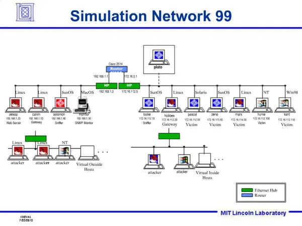
34. ns-2, the network simulator Our goal: • flavor of ns: simple example, modification, execution and trace analysis • discrete event simulator • modeling network protocols • wired, wireless, satellite • TCP, UDP, multicast, unicast • web, telnet, ftp • ad hoc, sensor nets • infrastructure: stats, tracing, error models, etc. • prepackaged protocols and modules, or create your own

35. “ns” components • ns, the simulator itself (this is all we’ll have time for) • nam, the Network AniMator • visualize ns (or other) output • GUI input simple ns scenarios • pre-processing: • traffic and topology generators • post-processing: • simple trace analysis, often in Awk, Perl, or Tcl • tutorial: http://www.isi.edu/nsnam/ns/tutorial/index.html • ns by example: http://nile.wpi.edu/NS/