Download

1 / 33
330 likes | 508 Views
Cost-based & Informed Search. Chapter 4. Review. We’ve seen that one way of viewing search is generating a tree given a state-space graph (explicitly or implicitly).

E N D
Cost-based & Informed Search Chapter 4
Review • We’ve seen that one way of viewing search is generating a tree given a state-space graph (explicitly or implicitly). • We’ve begun exploring various brute-force or uninformed methods of examining nodes [differentiated by the order in which nodes are evaluated] • The next wrinkle is to consider putting costs on the arcs
Search with costs • We might not be interested in finding the goal in the fewest number of hops (arcs) • Instead, we might want to know the cheapest route, even if it requires us to go through more nodes (more hops) • Assumption: the cost of any arc is non-negative • usually, this is thought of as distance from the start state
Uniform-cost search • Idea: the next node we are to evaluate is the node that is the cheapest to reach (in total cost) • the OPEN list should be sorted by cost (usually thought of as distance away from the start node) • produces the shortest path in terms of total cost • all the costs must be non-negative for this result to hold • usually called g(n) = cost of reaching node n • BFS produces the shortest path in terms of arcs traversed (BFS can be thought of as uniform-cost search with all arcs equal to one g(n) = depth(n)) [optimal] • this is not a heuristic search because we aren’t estimating a value; we know the cost exactly
Informal proof • If a lower-cost path existed, the beginnings of that path would already be in OPEN • But all of the paths in OPEN are at least as costly as the one popped off • This is because OPEN is kept sorted • Thus, since the cost function (g(n)) never decreases, we know that we’ve found the cheapest path
Bi-directional search • Can search from the start node to the goal • this is what we’ve been doing up until now • Can search from the goal to the start node • PROLOG does this, for instance • requires that we can apply our operators “backwards” • Split time working from both directions • fewer nodes overall should be expanded • example
Comparison of brute-force search • Fig. 3.18 • comparison factors • completeness: if a solution exists, is it guaranteed to be found • optimality: if a solution exists, is the best solution found? • space & time complexity: how much memory is required for the search? How long (on average) will the search take?
Summary of brute-force search • depth • breadth • iterative deepening • uniform cost • bidirectional
Growth of the CLOSED list • If OPEN can grow exponentially, can’t CLOSED as well? -Yes • for reasonable problems, we can use hash-tables; this just postpones the problem, however • we can also not use a CLOSED list • CLOSED prevents infinite loops, but if we’re using iterative deepening we don’t have this worry • obviously, if we’re using DFS this problem does arise & we have to try to avoid it by disallowing self-loops, for example (this doesn’t solve the whole problem, of course)
Best-first search (informed search) • We use some heuristic (evaluation (scoring) function) to determine which node to expand next • Incorporates domain specific knowledge and hopefully reduces the number of nodes we need to expand • Just as in the brute-force searches, however, we have to worry about memory usage • Use book slides on greedy search
Scoring functions • f(n) = g(n) + h(n) [general form] • g(n) = cost from start node to node n (current node) [we saw this in uniform-cost search] • important if we’re looking for the cheapest solution (optimal) and completeness • can also be used to break ties among h(n) values • h(n) = estimated cost to goal • heuristic • involves domain specific knowledge • should be quick & easy to compute
Heuristically finding least cost sol’n • g(n) alone produces the least-cost solution, but it doesn’t use heuristics to focus our efforts • solution: f(n) = g(n) + h(n) • how far we’ve come plus how much farther we think we have to go • combine the cost function (keeps the search “honest”) with the heuristic function (directs the search) • given certain restrictions on the heuristic function, we will still find the least-cost solution without (hopefully) expanding as many nodes as uniform-cost search
Using g(n) + h(n) • Keep the OPEN list sorted by f(n) = g(n) + h(n) • however, we must insure that if we come across some node N that is already on the OPEN list that the current cost of N isn’t less than the previous best cost for reaching N • if the current path to N is better, we delete the old node & add the new node because a better path has been found
Admissibility • Definition: if a search algorithm always produces an optimal solution path (if one exists), then the algorithm is called admissible. • If h(n) never over-estimates the actual distance to a node, then using f(n) = g(n) + h(n) will lead to an admissible best-first algorithm • called A* search • of course, it has the same drawbacks in terms of space as the other full search algorithms
More properties of A* • Domination: if h1, h2 are both admissible & h1(n) >= h2(n) for all n, then the nodes A* expands using h1 are a subset of those it expands using h2 • i.e., h1(n) would lead to a more efficient search • extreme case: h2(n) = 0 = no domain knowledge; any domain knowledge engineered into h1 would improve the search • we say that h1 dominates h2
Robustness • If h “rarely” overestimates the real distance by more than s, then A* will “rarely” find a solution whose cost is s more than the optimal • thus, it is useful to have a “good guess” at h
Completeness • A* will terminate (with the optimal solution) even in infinite spaces, provided a solution exists & all link costs are positive
Monotone restriction • If for all n, m where m is a descendent of n and h(n) - h(m) <= cost(n, m) [actual cost from going from n to m] • alternatively: h(m) >= h(n) - cost(n, m) • no node looks artificially distant from a goal • then whenever we visit a node, we’ve gotten there by the shortest path • no need for all of the extra bookkeeping to check if there are better paths to some node • extreme case: h(n) = 0 [then just BFS]
Creating heuristics [h(n)] • Domain or task specific “art” • A problem with less restrictions on the operators is called a relaxed problem. • It is often the case that the cost of an exact solution to a relaxed problem is a good heuristic for the original problem • example (8-puzzle)
Example heuristic • Domain: map • Heuristic: Euclidean distance • note that this will probably be an underestimation of the actual distance since most roads are not “as the crow flies”
Interesting problems are going to have very large search spaces & we may not be able to keep track of all possibilities on the OPEN list Further, sometimes we’re not interested in the single best answer (which might be NP-complete), but a “reasonably good answer” One method of doing this is to only follow the best arc out a given state if the next state is (judged to be) better than the current state & to disregard all the other children nodes Hill-climbing
Hill-climbing algorithm (partial) • Expanding a node, X • put X on CLOSED • let s = score(X) (usually smaller scores are best [estimating how far away from the goal we are] so we’re really doing “valley descending”) • consider the previously unvisited children of X • let C = best (lowest-scoring) child • let r = score(C) • if r s, then OPEN = { C } else OPEN = { } • I.e., continue as long as progress is being made • if no progress, simply stop (no backtracking)
Greedy algorithms • Hill-climbing is a greedy algorithm • It does what is locally optimal, even though a “less good” move may pay higher dividends in the future.
Uses of hill-climbing • Hill-climbing seems rather naïve, but it’s actually useful & widely used in the following type of situations • evaluating or generating a node is costly & we can only do a few • locally optimal solutions are OK • satisficing vs. optimal • e.g., decision trees and neural networks • constrained by time (the world might change while we’re thinking, for example) • we may not have an explicit goal test
Local maxima (optimality) • Local maxima • all local moves (i.e., all single-arc traversals form the current state) are lower than the current state, but there is a global maxima elsewhere • this is the problem with hill-climbing: it may miss global maxima
Beam search • Beam search also addresses the problem of large search spaces (keeping OPEN tractable) • However, instead of only putting the next best node on the OPEN list only if it is better than the current node • we will put the k best ones on OPEN • we will put them on OPEN regardless of whether they are better than the current node (this allows for “downhill” moves) • usually this technique is used with best-first search but it could be used with other techniques too -- in general, simply limit the OPEN list to k nodes
Partial v. full search tradeoffs • Partial -- don’t save whole space • hill-climbing, beam search • less storage needed (OPEN is limited in size) • faster; less nodes to search through • might miss (optimal) solutions since it is only considering part of the search space • Full -- ability to search whole space • DFS, BFS, best-first search
Simulated Annealing • Idea: avoid getting stuck in a local minima by occasionally taking a “bad” step • question: how often should we do this? • Too often & it will be just like a random walk • Reduce the probability of it happening as time goes on • analogous to molecules cooling • when heated they will be moving about randomly • as they cool, bonds start to form between them & the randomness decreases
SA algorithm • Extreme cases • temp is hot • e(energy / temp) goes to 1 • temp is cold • e(energy / temp) goes to 0 • becomes just like hill-climbing; no randomness any more
Search issues • Optimal v. any solution • huge search spaces v. optimality • cost of executing the search (the costs on the arcs) v. cost of finding the solution (arcs cost = 1) • problem specific knowledge v. brute-force • implicit v. explicit goal states