Download
1 / 35
350 likes | 416 Views
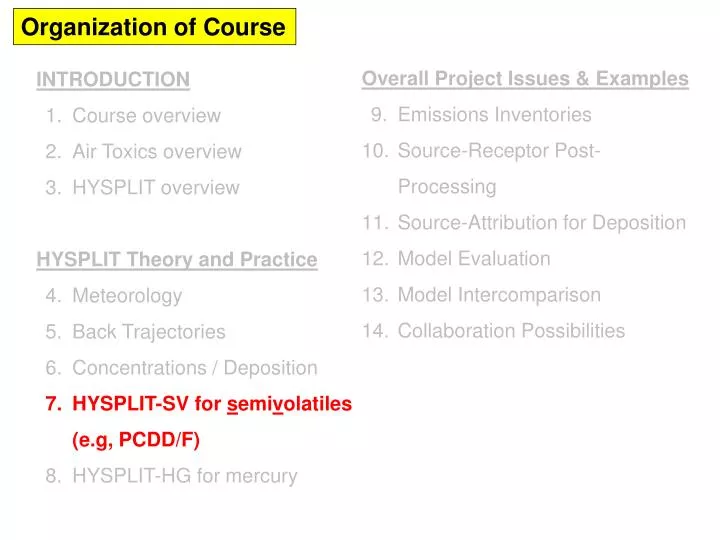
Organization of Course. Overall Project Issues & Examples Emissions Inventories Source-Receptor Post-Processing Source-Attribution for Deposition Model Evaluation Model Intercomparison Collaboration Possibilities. INTRODUCTION Course overview Air Toxics overview HYSPLIT overview

E N D
Organization of Course Overall Project Issues & Examples Emissions Inventories Source-Receptor Post-Processing Source-Attribution for Deposition Model Evaluation Model Intercomparison Collaboration Possibilities INTRODUCTION Course overview Air Toxics overview HYSPLIT overview HYSPLIT Theory and Practice Meteorology Back Trajectories Concentrations / Deposition HYSPLIT-SV for semivolatiles (e.g, PCDD/F) HYSPLIT-HG for mercury
210 Different Congeners, 17 are “toxic” 2,3,7,8-TCDD is believe to be the most toxic
Human exposure to dioxin is largely through food consumption, rather than from inhalation
In 1993, we obtained the HYSPLIT model (version 3) • Several modifications made to simulate PCDD/F & Hexachlorobenzene • Deposition accounting for specific point and area receptors • Vapor/particle partitioning for semivolatile compounds • Atmospheric chemistry – reaction with OH and photolysis • Particle size distribution for particle-associated material • Particle deposition estimated for each particle size • Enhanced treatment of wet and dry deposition • Accounting for five different deposition pathways • Dry -- gas • Dry -- particle • Wet -- below cloud high RH (droplets present below cloud) • Wet -- below cloud low RH (dry particles present below cloud) • Wet -- in cloud
Deposition from a given puff is assigned to a receptor, based on the overlap with that receptor, for each time step 10 1 2 6 4 5 3 11 12 7 8 9
C:\hysplit4\receptors\recp_data.txt minimum longitude of rectangle minimum latitude of rectangle maximum latitude of rectangle maximum longitude of rectangle 'Lake_Chapala‘, 1,-103.418,-103.343,20.223,20.289 / 'Lake_Chapala‘, 2,-103.343,-103.194,20.211,20.288 / 'Lake_Chapala‘, 3,-103.194,-103.085,20.163,20.285 / 'Lake_Chapala‘, 4,-103.085,-102.974,20.177,20.331 / 'Lake_Chapala‘, 5,-102.974,-102.766,20.173,20.311 / 'Lake_Chapala‘, 6,-102.766,-102.714,20.233,20.290 / 'Lake_Chapala‘, 7,-102.766,-102.693,20.173,20.211 / 'Lake_Chapala‘, 8,-102.861,-102.759,20.140,20.174 / 'Lake_Chapala‘, 9,-102.844,-102.803,20.111,20.140 / 'Lake_Chapala‘,10,-103.156,-103.085,20.285,20.324 / 'Lake_Chapala‘,11,-103.256,-103.194,20.180,20.211 / 'Lake_Chapala‘,12,-103.319,-103.256,20.199,20.211 /
You can add your own receptors! Also, in addition to “area” receptors, like a lake, point receptors can be added, e.g., corresponding to measurement site locations This is particularly useful for model evaluation
Fraction of emissions of four dioxin congeners accounted for in different fate pathways anywhere in the modeling domain for a hypothetical 1996 year-long continuous source near the center of the domain.
The fraction of emissions deposited does not drop off rapidly with distance… But, the deposition flux drops off very rapidly Logarithmic Deposition amount and flux of 2,3,7,8-TCDD in successive, concentric, annular 200-km-radius-increment regions away from a hypothetical 1996 year-long continuous source near the center of the modeling domain [40° N, 95° W).
Rate of destruction of PCDD/F congeners by photolysis is particularly uncertain…. To help understand uncertainties, sensitivity analyses can be very useful
Dry Deposition and Surface Exchange
Process Information: 1. Dry Deposition - Resistance Formulation • 1 • Vd = --------------------------------- + Vg • Ra + Rb + Rc + RaRbVg • in which • Ra = aerodynamic resistance to mass transfer; • Rb = resistance of the quasi-laminar sublayer; • Rc = overall resistance of the canopy/surface (zero for particles) • Vg = the gravitational settling velocity (zero for gases).
Dry Deposition • depends intimately on vapor/particle partitioning and particle size distribution information • resistance formulation [Ra, Rb, Rc...] • for gases, key uncertainty often Rc (e.g., “reactivity factor” f0) • for particles, key uncertainty often Rb • How to evaluate algorithms when phenomena hard to measure?
Particle dry deposition phenomena Atmosphere above the quasi-laminar sublayer Ra Very small particles can diffuse through the layer like a gas Very large particles can just fall through the layer Quasi-laminar Sublayer (~ 1 mm thick) In-between particles can’t diffuse or fall easily so they have a harder time getting across the layer Rb Wind speed = 0 (?) Rc Surface
Vd = settling velocity Diffusion low; Settling velocity low; Vd governed by Rb Diffusion high; Vd governed by Ra
More Information on Vapor / Particle Partitioning
In the atmosphere, pollutants can exist, generally, in the vapor phase or associated with particles, i.e., the aerosol phase. • For semivolatile compounds there can be there can be significant fractions associated with either phase. • This phenomenon is of crucial importance in determining the fate of semivolatile compounds in the atmosphere, because each of the deposition and destruction mechanisms depend a great deal on the physical form of the pollutant. • The vapor/particle partitioning phenomenon was first introduced by Junge (1977), and has been extended and reviewed by many…
The theory of vapor-particle partitioning postulates that for any species in the atmosphere, there is an equilibrium between vapor phase and the particle phase that depends primarily on: • the physical-chemical properties of the species of interest, • the nature of the atmospheric aerosol, • and the temperature.
As proposed by Junge (1977), the vapor-particle partitioning of exchangeable material can be estimated from the following equation: Φ = c St / (p(T) + cSt) where Φ = the fraction of the total mass of the species absorbed to the particle phase (dimensionless) St = the total surface area of particles, per unit volume of air (cm2/cm3) p(T) = the saturation vapor pressure of the species of interest (atm), at the ambient temperature (T) c = an empirical constant, estimated by Junge (1977) to be approximately 1.7 x 10⁻⁴ atm-cm
The most thermodynamically stable form of many semivolatile species at ambient temperatures is typically a solid, but, Bidleman (1988) has argued that it is the "non-equilibrium" or subcooled liquid phase which controls the dynamic equilibrium partitioning of such compounds between the vapor phase and the atmospheric aerosol. Thus, the subcooled liquid vapor pressure at the ambient temperature should be used in the above equation. This vapor pressure can be approximately estimated from the following equation: ln (Pl/Ps) = ΔSf (Tm - T) / RT where Pl = subcooled liquid vapor pressure (atm) at temp. T Ps = solid vapor pressure (atm) at temperature T ΔSf = entropy of fusion (atm m3/mole deg K) (approximately equal to 6.79 R) Tm = melting temperature of the solid compound (deg K) T = ambient temperature (deg K) R = the gas constant (atm m3/mole deg K)
The solid vapor pressure at the temperature of interest can be estimated from the reported solid vapor pressure at a standard temperature with the Clausius-Clapeyron equation using the enthalpy of vaporization, according to the following equation: ln (Ps1 / Ps2 ) = (ΔH / R) (1/T2 - 1/T1) where Ps1 = solid vapor pressure (atm) at temperature T1 Ps2 = solid vapor pressure (atm) at temperature T2 ΔH = enthalpy of vaporization (J/mole) Note: according to Trouton's Rule, ΔH can be approximately estimated by the following relation: ΔH /Tboil = 84 J/(mol degK) (Mackay et al 1986). R = gas constant (J/mole degK [=] (atm m3/mole deg K) T2 = temperature 1 (deg K) T1 = temperature 2 (deg K)
Thus, the vapor particle partitioning for a given compound in the atmosphere can be estimated from the first of the above two equations, with Pl from the second equation used for P(T). • The only species-specific physical-chemical property data required to make a vapor/particle partitioning estimate according to the above simplified approach are the species' solid vapor pressure at one temperature, and the species' boiling and melting temperatures.
It is typically assumed that semivolatile compounds in the atmosphere are "fully exchangeable", i.e., that the compound can move freely between the vapor and particle phases, depending on the dictates of thermodynamics. • To the extent that a portion of the material is "locked-up" within particles and is not available for exchange, this assumption would be in error.