Download
1 / 20
200 likes | 212 Views
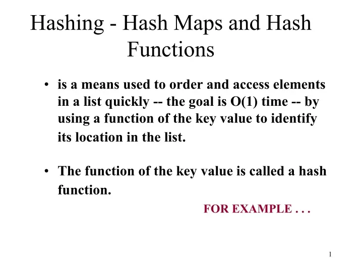
Hashing - Hash Maps and Hash Functions. is a means used to order and access elements in a list quickly -- the goal is O(1) time -- by using a function of the key value to identify its location in the list. The function of the key value is called a hash function. FOR EXAMPLE.

E N D
Hashing - Hash Maps and Hash Functions • is a means used to order and access elements in a list quickly -- the goal is O(1) time -- by using a function of the key value to identify its location in the list. • The function of the key value is called a hash function. FOR EXAMPLE . . .
Direct Address Tables If there is a collection of n elements whose keys are unique integers in (1, m), where m >= n, then we can store the items in a direct address table, T[m], where T[i] is either empty or contains one of the elements of our collection. Searching a direct address table is clearly an O(1) operation: for a key, k, we access T[k], if it contains an element, return it, if it doesn't then return a NULL. There are two constraints here:1) the keys must be unique, and 2) the range of the keys must be severely bounded.
If the keys are not unique, then we can simply construct a set of m lists and store the heads of these lists in the direct address table. The time to find an element matching an input key will still be O(1).
The range of the key determines the size of the direct address table and may be too large to be practical. For instance it's not likely that you'll be able to use a direct address table to store elements which have arbitrary 64-bit integers as their keys for a few years yet! Direct addressing is easily generalized to the case where there is a hash function, h(k) => (1, m) which maps each value of the key, k, to the range (1, m). In this case, we place the element in T[h(k)] rather than T[k] and we can search in O(1) time as before.
values [ 0 ] [ 1 ] [ 2 ] [ 3 ] [ 4 ] . . . Empty 4501 Empty 8903 8 10 7803 Empty . . . Empty 2298 3699 [ 97] [ 98] [ 99] A Simple (and poor) Hash Function HandyParts company makes no more than 100 different parts. But the parts all have four digit numbers. This hash function can be used to store and retrieve parts in an array. Hash(key) = partNum % 100
values [ 0 ] [ 1 ] [ 2 ] [ 3 ] [ 4 ] . . . Empty 4501 Empty 8903 8 10 7803 Empty . . . Empty 2298 3699 [ 97] [ 98] [ 99] Placing Elements in the Array Use the hash function Hash(key) = partNum % 100 to place the element with part number 5502 in the array.
Placing Elements in the Array values Next place part number 6702 in the array. Hash(key) = partNum % 100 6702 % 100 = 2 But values[2] is already occupied. COLLISION OCCURS [ 0 ] [ 1 ] [ 2 ] [ 3 ] [ 4 ] . . . Empty 4501 5502 7803 Empty . . . Empty 2298 3699 [ 97] [ 98] [ 99]
The direct address approach requires that the function, h(k), is a one-to-one mapping from each k to integers in (1, m). Such a function is known as a perfect hashing function: it maps each key to a distinct integer within some manageable range and enables us to trivially build an O(1) search time table. Unfortunately, finding a perfect hashing function is not always possible. Let's say that we can find a hash function, h(k), which maps most of the keys onto unique integers, but maps a small number of keys on to the same integer. If the number of collisions (cases where multiple keys map onto the same integer), is sufficiently small, then hash tables work quite well and give O(1) search times.
Handling the collisions In the small number of cases, where multiple keys map to the same integer, then elements with different keys may be stored in the same "slot" of the hash table. It is clear that when the hash function is used to locate a potential match, it will be necessary to compare the key of that element with the search key. But there may be more than one element which should be stored in a single slot of the table. Various techniques are used to manage this problem: chaining, overflow areas, re-hashing, using neighboring slots (linear probing), quadratic probing, random probing, ...
How to Resolve the Collision? values One way is by linear probing. This uses the rehash function (HashValue + 1) % 100 repeatedly until an empty location is found for part number 6702. [ 0 ] [ 1 ] [ 2 ] [ 3 ] [ 4 ] . . . Empty 4501 5502 7803 Empty . . . Empty 2298 3699 [ 97] [ 98] [ 99]
Resolving the Collision values Still looking for a place for 6702 using the function (HashValue + 1) % 100 [ 0 ] [ 1 ] [ 2 ] [ 3 ] [ 4 ] . . . Empty 4501 5502 7803 Empty . . . Empty 2298 3699 [ 97] [ 98] [ 99]
Collision Resolved values Part 6702 can be placed at the location with index 4. [ 0 ] [ 1 ] [ 2 ] [ 3 ] [ 4 ] . . . Empty 4501 5502 7803 Empty . . . Empty 2298 3699 [ 97] [ 98] [ 99]
Collision Resolved values Part 6702 is placed at the location with index 4. Where would the part with number 4598 be placed using linear probing? [ 0 ] [ 1 ] [ 2 ] [ 3 ] [ 4 ] . . . Empty 4501 5502 7803 6702 . . . Empty 2298 3699 [ 97] [ 98] [ 99]
Chaining for collisions (used in Lab 11) One simple scheme is to chain all collisions in lists attached to the appropriate slot. This allows an unlimited number of collisions to be handled and doesn't require a priori knowledge of how many elements are contained in the collection. The tradeoff is the same as with linked lists versus array implementations of collections: linked list overhead in space and, to a lesser extent, in time.
Clustering Linear probing is subject to a clustering phenomenon. Re-hashes from one location occupy a block of slots in the table which "grows" towards slots to which other keys hash. This exacerbates the collision problem and the number of re-hashes can become large.
Quadratic Probing Better behavior is usually obtained with quadratic probing, where the secondary hash function depends on the re-hash index: address = h(key) + c i2 on the ith re-hash. (A more complex function of i may also be used.) Since keys which are mapped to the same value by the primary hash function follow the same sequence of addresses, quadratic probing shows secondary clustering. However, secondary clustering is not nearly as severe as the clustering shown by linear probes.
Re-hashing schemes use the originally allocated table space and thus avoid linked list overhead, but require advance knowledge of the number of items to be stored. However, the collision elements are stored in slots to which other key values map directly, thus the potential for multiple collisions increases as the table becomes full.
Overflow area Another scheme will divide the pre-allocated table into two sections: the primary area to which keys are mapped and an area for collisions, normally termed the overflow area.
When a collision occurs, a slot in the overflow area is used for the new element and a link from the primary slot established as in a chained system. This is essentially the same as chaining, except that the overflow area is pre-allocated and thus possibly faster to access. As with re-hashing, the maximum number of elements must be known in advance, but in this case, two parameters must be estimated: the optimum size of the primary and overflow areas.