Download
1 / 30
300 likes | 370 Views
Andrei Poblaguev 09 / 13 / 2010. Comments to the AGS pC polarimeter data processing. t 0 based calibration Observations of Boris Morozov’s results

E N D
Andrei Poblaguev 09 / 13 / 2010 Comments to the AGS pCpolarimeter data processing • t0 based calibration • Observations of Boris Morozov’s results • Dead layer corrections. A novel method of calibration. • Algorithm for the WFD firmware
t0 based calibration A. Poblaguev
Introduction • Measured values: • tm → t = tm-t0 • A → W = kA → E = E(xdl ,W) • Calibration parameters: • k - amplitude calibration • xdl - (effective) dead layer • t0 - mean time of proton interaction with the target. • L - distance from the target to the detector. • Basic assumptions and definitions: • t is time-of-flight • E= (ML2/2) / t2 is Carbon energy (in the target) • W is measured energy (good accuracy but E nonlinearly depends on W). • Big fluctuations in tm values due to the “bunch width”. • No systematic errors in measurements of time and Amplitude. A. Poblaguev
Time distributions for fixed Amplitude Amplitudes are measured as a set of discrete values. Every histogram is for given amplitude value. A. Poblaguev
Mean Time vs Amplitude • mean timevsamplitude for the energy range 400-900 keV(according to the calibration in the data file) • mean time vsamplitude for other energies A. Poblaguev
Time based calibration of the measured amplitude If t0 is known we can calibrate amplitude using experimental data: E = E(A) After that the amplitude may be used to measure energy with good accuracy and the time may be used to cut background only. • With known t0 we do not need other calibrations (alpha, dead layer) any more • However other calibrations are important tool to verify results of measurements. A. Poblaguev
Comparison with existing calibration (from the file) A. Poblaguev
Observations of Boris Morozov’s results A. Poblaguev
Boris Morozov’s results The total background level ~ 12%. (B.M.) • Is horizontal line “the photon prompt”? • Why background is suppressed in Boris’es measurements ? • Misinterpretation ? • Different detector ? • Errors in WFD firmware ? A. Poblaguev
Some results from tandem tests (B.M.) Significant background in BNL detector response ! Alpha Calibration + “standard” deadlayer correction may not work perfectly at low energies. A. Poblaguev
Dead Layer corrections.A novel method of calibration. A. Poblaguev
Time vs Time plot A→W = kA → E = E(xdl ,W) →τ = L√ M/2E • Advantage of the time/time plot: • straight line • 45 degree slope • t0 variation is separated from k and xdl. • How calibration fit works: • The experimental line is transformed to the strait one by variation the xdl (or k) • check the 45 degree condition • find t0 t0 • The τ dependence on both xdl and k is well approximated by linear transformation • τ→τ + (a+bτ) δp, p=xdl,k • (for the considered energy range). • Essential nonlinearity for the data. A. Poblaguev
45 degree view For proper calibration, (vertical) strait line is expected . Not the case A. Poblaguev
Explanation of the picture • Two strait lines may be found: • 400 – 900 keV • 650 – 1200 keV • More likely that 650-1200 keVcalibration is correct: • Better accuracy of measurements • xdlcorrection is less dependent on accuracy of knowledge of dE/dx: • - relatively (variations of dE/dx) • - absolutely (dead layer/total path ratio) • xdl corrections do not work perfectly if E<600 keV. • systematic error in energy measurement up to 5% A. Poblaguev
Similar effect in other channels/runs A. Poblaguev
The effective dead layer EL E0 x0x0+Δ xdl Generally xdl depends on energy. The dependence may be “compensated” by variations of dE/dx. A. Poblaguev
Can we measure dE/dx ? In the effective dead layer approximation: xtot(E) –xtot(W) = xdl = 1 (if length is measured in units xdl) In experimental data we have set (continium) of pairs (Ei, Wi) where iis the event number. F(E) = x(E) + const F(E0 ) –F(W0) = 1 F(E1=W0) –F(W1) = 1 F(E2=W1) –F(W2) = 1 …. The set of points with energies E0,E1,E2,… is on the F(E) with the displayment of 1. A. Poblaguev
Results for the effectivedE/dx(Very preliminary. Tuning is needed) F(E) = xtot(E) = p1*E + p2*E2 + … + pnPar*EnPar We can find pi by minimization of Σ [ F(p,Ei) – F(p,Wi) – 1 ]2 dE/dx = dF(p,E)/dE E = F-1[ F(W) + 1 ] A. Poblaguev
Did it help ? • Calibration made with one strip is applicable to other strips • (but may require adjustment of dead layer thickness) • For the strip #6, the effective dead layers in runs 42500 and 42600 differ by about 10%. A. Poblaguev
Can we measure t0, k, L from data? • The dE/dx fit works well if t0 and k are known • This is a partial (parameterized) case of the general t0 based calibration • A special fit (minimization of the χ2) is needed to find t0, k, and L. A. Poblaguev
The Fit • Preliminary results are • optimistic • (we do not need to know dE/dx, α-calibration, and even distance between target and detector, all calibrations may be extracted from the data) • More study is needed to prove the method and to understand systematic errors. Search for alphas might be a powerful stress-test for the method. A. Poblaguev
Algorithm for the WFD firmware A. Poblaguev
Existing WFD firmware algorithm Smoothed signal • Actually, 140 MHz WFD (7 ns) • Effectively (3 “colors”) 420 MHz WFD (2.4 ns) • Baseline depends on color (?) • Gain depends on color (?) • Firmware algorithm (my understanding) • Signal smoothing: ai → ãi = (ai-1 + ai + ai+1) ∙5/16 • Searching for baseline • Searching for signal maximum • Time determination (at half maximum with step ~ 1.2 ns) • Four byte output: Tmax, t, A, Int (+ event identification) RHIC Yellow Data Restored color signals Effectively 6-bit WFD (after conversion) ai+3 = ai + (ãi+2 – ãi+1) ∙ 16/5 A. Poblaguev
A possible weakness of the algorithm • Factor 5/16 in smoothing → oscillations in measured amplitude • Oscillations in measured time • Do baseline fluctuations properly controlled ? A. Poblaguev
One “color” measurements (140 MHz mode) • Previous experience: • In KOPIO we had time resolution ~ 200 ps with the same WFD (140 MHz mode) • In ATLAS ZDC we have time resolution ~ 200 ps with 40 MHz WFD by measuring ratio of 2 amplitudes Am-1/Am Time-slice amplitude ratio may be used to measure time: (Tmax, t, Amp, Int) (m, Am-1, Am , Am+1) ↓ (offline) Baseline, Amplitude, Time A. Poblaguev
Time from Amplitude Ratio • Amplitude ratio distributions t(r=0.16) = 14 ns t(r=0.54) = 7 ns t(r=1.00) = 0 ns t(r=1.39) = -7 ns (Linear approximation) t(r) = (1-r)/0.46 * 7 ns Definitions Polinomial fit: t = P(r) = p1(1-r) + p2(1-r)2 +… by minimization of Σ [ t(rm-1)-t(rm) -7 ns ]2 A rectangular shape indicates goog time resolution and good linearity A. Poblaguev
Time difference between “colors” Linear Calibration: Actual signals derived from the smoothed ones. Factor 3 degradation is expected due to the conversion. Smoothed signals. • Run average baseline value was used in calculations • Amplitude range: 30-200 WFD counts • Actual single color time resolution may be factor 1/√2 better (if no correlation between “colors”) A. Poblaguev
Time difference between “colors” Polinomial Calibration: Actual signals derived from the smoothed ones. Factor 3 degradation is expected due to the conversion. Smoothed signals. Actually no improvement compared to the linear calibration! A. Poblaguev
Suggestion for new firmware(single “color”) • Time resolution in 140 Mhz WFD is better than 200 ps (for the amplitude range of 30 – 200 WFD counts . • Optimization of baseline measurements to be studied. • Corrections to the Signal amplitude to be studied. • Best solution: Firmware returns(m, p, Am-1, Am, Am+1) • (require extra byte for every event, but offline data • contains sufficient information for the calibration and • “corrupted” events suppression) • Good solution: (m, Am-1, Am, Am+1)or (m, Am-2, Am-1, Am) • (applicable only if baseline could be properly calculated • from the amplitudes.) • Satisfactory solution: (m, p, Am-1, Am) • Minimal solution:(m, Am-1-p, Am-p) m - index of the maximum amplitude p - the baseline value calculated in firmware Ak - raw amplitudes More study with true raw data is needed ! A. Poblaguev
Summary • Measurement and monitoring of t0 allows us to make a model independent calibration of the polarimeter • Other methods of calibration are needed to verify results. • The MSTAR dE/dx does not fit data well. • Up to 5% inaccuracy in energy measurements. • Calibration in 0.65-1.2 MeV region may help ! • A novel method of calibration is suggested: • We do not need 3 “colors” in WFD. • 140 MHz WFD allows us to measure time with accuracy better than 200 ps. • Understanding of baseline calibration/determination is still needed. • More simple firmware might be more efficient. • Dead layer corrections as well as the calibration parameters • t0, k, L may be evaluated from the data. • No special calibration needed. • Study of the systematic errors is needed. A. Poblaguev