Download
1 / 24
240 likes | 375 Views
Simulations of Stochastic Biological Phenomena. Fernand Hayot, PhD Department of Neurology Mount Sinai School of Medicine fernand.hayot@mssm.edu. 1. Part 1 . Modeling Stochastic Systems: The Master Equation.

E N D
Simulations of Stochastic Biological Phenomena Fernand Hayot, PhD Department of Neurology Mount Sinai School of Medicine fernand.hayot@mssm.edu 1
Part 1. Modeling Stochastic Systems: The Master Equation Measurements on single cells rather than across a population of cells: emphasis on variability from cell to cell, rather than on average behavior. Importance: Cell variability can lead to different phenotypic outcomes; average behavior can mask what actually happens in individual cells, such as graded average response masking all-or-none individual cell response. Example: Ferrell JE Jr, Machleder EM. The biochemical basis of an all-or-none cell fate switch in Xenopus oocytes. Science. 1998 May 8;280(5365):895-898. PMID: 9572732 2
Responses to progesterone stimulation of individual oocytes Ferrell JE Jr, Machleder EM. The biochemical basis of an all-or-none cell fate switch in Xenopus oocytes. Science. 1998 May 8;280(5365):895-898. PMID: 9572732 3
Why do we need to consider stochasticity? , i.e. i.e. , i.e., (stochasticity=randomness=fluctuations) Example: Consider a collection of p identical proteins that decay at a rate k, which means that per unit time k proteins disappear. Deterministically However the decay process is stochastic: each protein has a probability kdt to decay in the time interval (t, t + dt). 4
Why do we need to consider stochasticity? (stochasticity = randomness = fluctuations) Example (continued): Now consider N boxes, each one with the identical system of p proteins, all having the same initial number p(0) and decaying at the same rate k. Suppose I open the boxes some time later and check the number of proteins: I'll find different numbers in each box, differing by small amounts. • If the numbers are large, these differences do not matter, and the deterministic equation is a good description of what happens in each box. • However, when the number of initial proteins is small, say 10, the differences matter, the effect of the stochasticity of the decay shows up, and the deterministic approach to each box is no longer appropriate. 5
Why do we need to consider stochasticity? Example details N identically prepared cells, numbered i = 1,2,...N At some time t, measurethe copy number xiof some protein or mRNA in each cell One can define: average: <x> = (x1+ x2 + ............ xN)/ N variance:σ2 = <x2> – <x>2 = < (x – <x>)2> Standard deviation = σ; coefficient of variation= σ/<x>; Fano factor= σ2/<x> 6
Why do we need to consider stochasticity? Example details N large: statistical interpretation Histogram: number of cells for which xi lies in some small interval x < xi< x + δx Histogram is an approximation (better the larger N) to the probability density distribution of the number of measured protein or mRNA across the N cells. Knowledge of <x> and σ (better the complete probability distribution) allows comparison with known distributions: Poisson, Gaussian, gamma, lognormal. 7
Noise in protein levels in yeast cells The figure shows several genes, conditions and time points. Thick line in (a): log (σ2/<p>2) = 1175 – log(<p>) Thin line in (b) is autofluorescence: log (σ2/<p>2) = 9.9 .105 – 2 log(<p>) Thus, slope of autofluorescence is twice slope of thick line Bar-Even A, Paulsson J, Maheshri N, Carmi M, O'Shea E, Pilpel Y, Barkai N. Noise in protein expression scales with natural protein abundance. Nat Genet. 2006 Jun;38(6):636-43. PMID: 16715097 8
Deterministic versus stochastic representations Birth-and-Death Process: transcription and mRNA degradation Model: D→ D + M, rate k1; M → Ф, rate k3 D = DNA M = mRNA Φ = degradation product ODE for concentrations: This works well for cell population average, or for a single cell when the number n of M is so large that any change to it from the above reactions (change of +1 or –1) can be treated differentially. If n is small (say of the order of 100 and less), one has what is called “small copy number” fluctuations, and the appropriate language now becomes that of probabilities. 9
Deterministic versus stochastic representations The new quantity now is P(n,t), the probability of having n copies of M in the cell at time t. This probability satisfies an evolution equation called the Master equation. For the above birth-and-death process this equation is How does this equation come about? 10
Derivation of the Master Equation Model: D→ D + M, rate k1; M → Ф, rate k3 D = DNA M = mRNA Φ = degradation product Take time interval δt sufficiently small so that either none of the 2 reactions takes place, or a single reaction, but not 2. Then ask for P(n, t + δt), knowing the state of the cell at time t. 3 contributions between t and t + δt: - “birth” takes place: k1 δtnDP(n – 1, t) - “death” takes place: k3 δt (n + 1) P(n + 1, t) - no reaction occurs: (1 – k1 δtnD – k3 δtn) P(n,t) 11
Derivation of the Master Equation Put nD=1; one promoter-transcription factor complex (haploid cell) Now put P(n,t+δt) equal to the 3 contributions, replace [P(n,t+δt)-P(n,t)]/δt by ∂P(n,t)/∂t and the full Master equation of the preceding slide is obtained, namely 12
Calculate average of n from Master equation: Average: multiply Master equation by n, and sum over all n, using Σ P(n,t)=1, Σ n P(n,t)= <n(t)> d <n(t)>/dt = k1 – k3 <n> Result: the average value <n(t)> follows the same equation as the concentration [M(t)] of the ODE equation. Additional hints relevant to Problem Set If we multiply the Master equation by n2 and sum, this results in an equation for the variance. The steady-state relation between mean and variance provides important information. Consider the steady state of the Master equation: ∂P(n,t)/∂t =0, and (n+1)P(n+1)=nP(n)+ (k1/k3) [P(n)-P(n-1)]. Notice that P(n+1) is determined, once P(n) and P(n-1) are known. Therefore, one can find the steady state solution recursively, starting with P(1) (on the LHS) , with P(-1)=0. 13
A model of transcription plus translation The model of transcription and mRNA degradation was expanded: Thattai M and van Oudenaarden A, PNAS 2001 98:8614-8619. Model of Transcription & mRNA degradation only: D→ D + M, rate k1 M → Ф, rate k3 Complete Model: D→ D + M, rate k1 M→ M + P, rate k2 M → Ф, rate k3 P → Ф, rate k4 The Problem Set requires exploring this model 14
Part 2. Modeling Stochastic Systems: The Gillespie Algorithm 15
Master equation in most cases is too complicated to be dealt with directly. Gillespie's algorithm is a numerical scheme that is equivalent to solving the Master equation. The crux of the algorithm is the drawing of 2 random numbers at each time step, one to determine when the next reaction among the reactions considered will take place, the second one to choose which one of the reactions will occur. Suppose there are j = 1,2,.... reactions. Given the state of the system at time t, aj(t)dt denotes the probability that reaction j will occur in the time interval (t, t + dt). aj(t) is the product of 2 parts: reaction rate cj for reaction j, and the number of possible reactions in volume V. Gillespie DT. Exact stochastic simulation of coupled chemical reactions. J. Phys. Chem. 1977;81, 2340-2361. Gillespie DT. Approximate accelerated stochastic simulation of chemically reacting systems. J. Chem Phys. 2001115, 1716-1733. 16
Example: dimerization reaction P1 + P2 → Z, rate cj Here aj(t) = cj P1(t) P2(t), where P1(t) P2(t) represents the product of the numbers of molecules of P1 and P2 at time t. If P2 identical to P1 then aj(t) = cj P1(P1 – 1)/2 Remark: connection between the c's and the corresponding chemical rate constants k's that appear in the ODEs (This remark applies as well to the Master Equation derivation) By definition the c's have dimension of inverse of time. When the chemical rate constant has the dimension of an inverse time as is the case for the transcription-translation-degradation model considered previously, then c is equal to k. However for the above dimerization reaction, one would have the ODE d[Z]/dt = k[P1][P2], where k has dimension of volume over time. In this case c = k/V (c = 2k/V if P1 = P2), V representing the volume where the reaction takes place (whole cell, cytoplasm, nucleus) (1 nM corresponds to 1 particle in a volume of 1.6 micron cube.) 17
Implementation of Gillespie’s Algorithm At time t the number of molecules of each of the interacting species are known, the aj(t) are known. Call ao(t) = Σaj(t). Take the following steps: 1. Find time τ at which the next reaction takes place; draw random number from an exponential probability distribution p(τ)= ao exp(-ao τ) 2. Choose what reaction takes place at time τ; draw a random number from a uniform distribution between 0 and 1. If that number falls between 0 and a1/ao, reaction 1 is chosen, between a1/ao and (a1 + a2)/ao reaction 2, and so on. 3. The occurrence of the chosen reaction changes the numbers for the molecules involved, for example for the dimerization reaction P1→P1 – 1, P2→ P2 – 1, Z→ Z+1. Consequently the value of the corresponding aj(t + τ) is different from aj(t). 4. Reiterate, starting from point 1, as long as one wishes to follow the evolution of the system 18
Remarks in connection with Gillespie’s algorithm implementation If 2 random numbers x and y are connected through a monotonic function, such that y = f(x), then knowing the probability density function of x, namely p(x), one finds p(y) = p(x) |dx/dy| For instance, if x is uniformly distributed between 0 and 1, then y = –(log x)/a is exponentially distributed. Why is τ exponentially distributed? System known at time t. Probability that the next reaction occurs between t + τ and t + τ + dτ p(τ) dτ = p(no reaction between t and t + τ) x p(reaction between t + τ and t + τ + dτ) p(τ) dτ = exp(-ao τ) ao dτ 19
A MATLAB implementation of Gillespie’s algorithm % intialization of components d=1; r=0; time=0; timelimit= 500 ; % Main loop over time while time < timelimit a1=k1*d ; a2=k3*r ; a0=a1+a2 ; r1=rand ; r2=rand ; tau=-(1./a0)*log(r1) ; yr2=r2*a0 ; cumprobs = zeros(1,3) ; cumprobs(2)=cumprobs(1)+a1 ; cumprobs(3)=cumprobs(2)+a2 ; for k=2:length(cumprobs) if ( (cumprobs(k) >= yr2) & (cumprobs(k-1) < yr2) ) mu=k-1; end end if (mu == 1) r = r + 1 ; end if (mu == 2) r = r - 1 ; end time=time+tau; end core_gillespie.m Reactions: D→ D + M, rate k1 M→Ф ,rate k3 r = # mRNA molecules Choice of time limit? Need to know k1,k3 take k1=0.01 1/s k3=0.0058 1/s characteristic times: t1= 1/c1=100 s t3= 1/c3= 172 s 20
Some remarks on Gillespie's program Efficiency: several tens of reactions problem of very fast time scales Acceleration of Gillespie's algorithm for large systems: “tau leap” algorithm Gillespie DT and Petzold LR, J. Chem. Phys. 2003;119, 583-591. Gibson-Bruck algorithm Gibson MA and Bruck J, J. Phys. Chem. A 2000; 104, 1876-1889. Software packages: “Dizzy” Ramsey et al., J. Bioinf. Comp. Biol. 2005 3, 415-436. Hybrid models: combining deterministic and stochastic simulations 21
REMARKS ON NOISE: Intrinsic and Extrinsic Noise Until now: small copy number noise:Intrinsic noise. Extrinsic noise: example: cell-to-cell variability of a kinase activated by a stimulus Other source of Intrinsic noise: transcription and transcriptional bursting Example Human dendritic cells infected by virus exhibit transcriptional bursting Examine cell-to-cell variability in IFNβ (interferon beta) mRNA This is evident in a log-log plot of mRNA versus cumulative probability Simulation Results Experimental Data Hu J et al.. Power-laws in interferon-B mRNA distribution in virus-infected dendritic cells Biophys. J. 2009 97, 1984-1989. 22
REMARKS ON NOISE: Intrinsic and Extrinsic Noise Model of transcriptional bursting to explain IFNβ mRNA levels in infected dendritic cells Simplified model D+P1 ↔ Ds1 Ds1+P2 ↔ Ds11 Ds11 ↔ D* D* → D* + M M → 0 P1 and P2 transcription factors whose binding leads to Ds11. Stochastic TF binding (reactions 1 and 2) coupled to random bursting (reactions 3 to 5). References: J. Hu, S.I. Biswas, S.C. Sealfon, J. Wetmur, C. Jayaprakash, F. Hayot, Biophys. J. 97, 1984- 1989 (2009) S. Iyer-Biswas, F. Hayot, C. Jayaprakash, Phys. Rev. E, 031911 (2009) J. Hu, S. Sealfon, F. Hayot, C. Jayaprakash, M. Kumar, A.C. Pendleton,A. Ganee, A. Fernandez-Sesma, T.M. Moran, and J.G. Wetmur, Nucleic Acids Res, 35, 5232-5241 (2007) 23
Slides from a lecture in the course Systems Biology—Biomedical Modeling Citation: F, Simulations of stochastic biological phenomena. Sci. Signal.4, tr13 (Citation: F. Hayot, Stimulations of stochastic biological phenomenon. Sci. Signal. 4, tr13(2011).). www.sciencesignaling.org