Download
1 / 26
2.33k likes | 5.12k Views
5.4.3 Round Robin Scheduling. A preemptive scheduling designed for Time Sharing Systems The Ready Queue is treated as a circular queue A small execution time interval is defined as the Time Quantum, or time slice. Interrupts in Round Robin.

E N D
5.4.3 Round Robin Scheduling • A preemptive scheduling designed for Time Sharing Systems • The Ready Queue is treated as a circular queue • A small execution time interval is defined as the Time Quantum, or time slice
Interrupts in Round Robin • When the executing interval of a process reaches the time quantum, the timer will cause the OS to interrupt the process • The OS carries out a context switch to the next selected process from the ready queue.
Length of the Time Quantum • Time quantum that is too short will generate many context switching and results in lower CPU efficiency. • Time quantum that is too long may result in poor performance time.
RR Scheduling (cont’d) Example: Five processes arrive at time 0, in the order: P1, P2, P3, P4, P5. Their CPU burst time are shown in the following table. Using RR with Quantum =40 msec, find the average turnaround time and average waiting time
Fourth round (fourth turn): 518 to 566 ms Average Turnaround Time = (Ta(P3)+Ta(P2) +Ta(P1)+Ta(P4)+Ta(P5)) / 5 = (296+438+533+561+566) / 5 = 478.8 ms
Example with Round Robin The chart for Round-Robin, with Quantum =40 msec., is:
Wait Time: Average Wait Time = (Tw(P1)+Tw(P2) +Tw(P3)+Tw(P4)+Tw(P5)) / 5 = (398+336+240+413+441) / 5 = 365.6 ms
5.4.4 Shortest Remaining Time First • Shortest remaining time (SRTF) is a preemptive version of SPN scheduling. • With this scheduling policy, a new process that arrives will cause the scheduler to interrupt the currently executing process if the CPU burst of the newly arrived process is less than the remaining service period of the process currently executing. • There is then a context switch and the new process is started immediately.
SRTF Scheduling • When there are no arrivals, the scheduler selects from the ready queue the process with the shortest CPU service period (burst). • As with SPN, this scheduling policy can be considered multi-class because the scheduler gives preference to the group of processes with the shortest remaining service time and processes with the shortest CPU burst.
SRTF Example Process Arrival time CPU burst P1 0 135 P2 0 102 P3 0 56 P4 0 148 P5 0 125 P6 200 65
Gantt Chart for SRTF Example Turnaround Time: Ta(p3)=56, Ta(p2)=56+102=158 At time 200, P5 has executed during 42 msec and has remaining service time of 83 microseconds, which is greater than the CPU burst of P6 (i.e., 65 ms). Ta(p6) = 65, Ta(P5)= 56+102+42+65+83=348 Ta(P1) = 348+135 = 483 Ta(P4) = 483 + 148 = 631
Results of Example Using SRT Process Start Completion Wait Turnaround Ntat P1 348 483 348 483 3.577 P2 56 158 56 158 1.549 P3 0 56 0 56 1.0 P4 483 631 483 631 4.263 P5 158 348 223 348 2.784 P6 200 265 0 65 1.0 The average wait period = (248+56+0+483+223+0)/6=185.0 microsec. The average turnaround time = (483+158+56+631+348+65) =290.16 microsec.
5.4.6 Dynamic Priority Scheduling • Processes that request I/O service will typically start with CPU service; for a short time; request another I/O operation; and release the CPU. • If these processes are given higher priority, they can keep the I/O devices busy without using a significant amount of CPU time. • This will tend to maximize I/O utilization while using a relatively small amount of CPU time. • The remaining CPU capacity will be available for processes that are requesting CPU bursts.
Dynamic Priority Scheduling (2) • The CPU scheduler dynamically adjusts the priority of a process as the process executes. • The typical approach is to adjust the priority based on the level of expectation that the process will carry out a system call (typically an I/O request). • However, this requires the CPU scheduler to predict future process requests.
5.4.7 Other Scheduling Policies5.4.7.1 Longest Process Next Not attractive
5.4.7.2 Real-Time Systems • A system that maintains an on-going interaction with its environment • One of the requirements of the system is its strict timing constraints • The system depends on priorities and preemption
Real-Time Scheduling Policies • One of the goals of real-time scheduling is to guarantee fast response of the high-priority real-time processes. • The second general goal is to guarantee the processes van be scheduled in some manner to meet their individual deadline.
Real-time Processes • The real-time processes, each with its own service demand, priority and deadline, compete for the CPU. • Real-time processes must complete their service before their deadlines expire. • The performance of the system is based on this guarantee.
Real-time Processes (2) • The real-time processes can be: • Periodic processes need to be executed every specific interval (known as the period) • Sporadic processes can be started by external random events. • The operating system uses a real-time scheduling policy based on priorities and preemption.
5.5 Multiple Processors • For multiple-processor systems, there are several ways a system is configured. • More advanced configurations and techniques for example, parallel computing, are outside the scope of this book.
5.6 Summary • FCFS • SJF • RR • SRT