Download
1 / 54
540 likes | 574 Views
2. Differentiable Manifolds And Tensors. 2.1 Definition Of A Manifold 2.2 The Sphere As A Manifold 2.3 Other Examples Of Manifolds 2.4 Global Considerations 2.5 Curves 2.6 Functions On M 2.7 Vectors And Vector Fields 2.8 Basis Vectors And Basis Vector Fields 2.9 Fiber Bundles

E N D
2. Differentiable Manifolds And Tensors 2.1 Definition Of A Manifold 2.2 The Sphere As A Manifold 2.3 Other Examples Of Manifolds 2.4 Global Considerations 2.5 Curves 2.6 Functions On M 2.7Vectors And Vector Fields 2.8 Basis Vectors And Basis Vector Fields 2.9 Fiber Bundles 2.10 Examples Of Fiber Bundles 2.11 A Deeper Look At Fiber Bundles 2.12 Vector Fields And Integral Curves 2.13 Exponentiation Of The Operator d/d 2.14 Lie Brackets And Noncoordinate Bases 2.15 When Is A Basis A Coordinate Basis?
2.16 One-forms 2.17 Examples Of One-forms 2.18 The Dirac Delta Function 2.19 The Gradient And The Pictorial Representation Of A One-form 2.20 Basis One-forms And Components Of One-forms 2.21 Index Notation 2.22 Tensors And Tensor Fields 2.23 Examples Of Tensors 2.24 Components Of Tensors And The Outer Product 2.25 Contraction 2.26 Basis Transformations 2.27 Tensor Operations On Components 2.28 Functions And Scalars 2.29 The Metric Tensor On A Vector Space 2.30 The Metric Tensor Field On A Manifold 2.31 Special Relativity
2.1. Definition of a Manifold Rn Set of all n-tuples of real numbers A ( topological ) manifold is a continuous space that looks like Rn locally. Definition: ( Topological ) manifold A manifold is a set M in which every point P has an open neighborhood U that is related to some open set fU(U)of Rn by a continuous 1-1 onto map fU. Caution: Length is not yet defined. xUj(P) are the coordinates of P under fU. Dim(M) = n. M is covered by patches of Us. Subscript U will often be omitted
Let be 1-1. (U, f ) = Chart U,V open open Let ( Coordinate transformation ) Charts (U, f ) & (V, g ) are Ck - related if exist & are continuous i, j
Atlas = Union of all charts that cover M M is a Ck manifold if it is covered by Ck charts. A differentiable manifold is a Ck manifold with k > 1. • Some allowable structures on a differentiable manifold: • Tensors • Differential forms • Lie derivatives M is smooth if it is C. M is analytic (C) if all coordinate transformations in it are analytic functions.
2.2. The Sphere As A Manifold Every P has a neighborhood that maps 1-1 onto an open disc in R2. ( Lengths & angles not preserved ) Spherical coordinates: • Breakdowns of f : • North & south poles in S2 mapped to line (0, x2) & (, x2) in R2, resp. • Points (x1, 0) & (x1, 2) correspond to same point in S2. 2nd map needed Both poles & semi-circle joining them ( = 0 ) not covered
One choice of 2nd map: Another spherical coordinates with its = 0 semi-circle given by { (/2 , ) | {/2 , 3/2 } } in terms of coordinates of 1st system. Stereographic map (fails at North pole only) North pole mapped to all of infinity These conclusions apply to any surface that is topologically equivalent to S2. The 2-D annulus bounded by 2 concentric circles inR2 can be covered by a single ( not differentiable everywhere ) coordinate patch
2.3. Other Examples Of Manifolds Loosely, any set M that can be parameterized continuously by n parameters is an n-D manifold • Examples • Set of all rotations R(,,) in E3. ( Lie group SO(3) ) • Set of all boost Lorentz transformations (3-D). • Phase space of N particles ( 6N-D). • Solution space of any ( algebraic or differential ) equation • Any n-D vector space is isomorphic to Rn. • A Lie group is a C-manifold that is also a group. Rn is a Lie group wrt addition.
2.4. Global Considerations Any n-D manifolds of the same differentiability class are locally indistinguishable. Let f: M N If f & f –1 are both 1–1 & C, then f is a diffeomorphism of M onto N. M & N are diffeomorphic. • Example of diffeomorphic manifolds: • Smooth crayon & sphere • Tea cup & torus
2.5. Curves Parametrized curve with parameter
2.6. Functions on M f is differentiable if f(x1,…,xn) C1 Reminder: Any sufficiently differentiable set of equations that is locally invertible ( with finite Jacobian ) is an acceptable coordinate transformation
2.7. Vectors and Vector Fields Let be a curve Cthrough P on M. be a differentiable function on M. is a differentiable function on C. Chain rule: { d xi }= infinitesimal displacement along C d xi components of vector tangent to C = vector tangent to C with components wrt basis Tangent (vector) space TP(M) at P :
Advantages of defining vector as d/d: • No finite distance involved works on manifolds without metric. • Coordinate free. • Conforms with the geometric notion that a tangent is generated by some infinitesimal displacement along the curve. • Finer points: • Each d/d denotes an equivalent class of diistinct curves having the same tangent at P. • Two vectors d/d & d/d may denote the same tangent to the same curve under different parametrization. • Only vectors at the same point on M can be added to produce another vector. ( Vectors at different points belong to different vector spaces )
2.8. Basis Vectors And Basis Vector Fields • Let M be an n-D manifold. • P M, TP(M)is an n-D vector space. • Any collection of n linearly independent vectors in TP(M) is a basis for TP(M). • A coordinate system { x i} in a neighborhood U of P defines a coordinate basis { / x i } at all points in U. Let be an arbitrary (non-coordinate) basis for TP(M). For a vector field, V i & V j are functions on M. The vector field is differentiable if these functions are.
{ / x i } is a basis it is a linearly independent set. This is guaranteed if { x i } are good coordinates at P. Proof: Let { y i } be another set of good coordinates at P. is invertible Inverse function theorem i.e., vectors with components given by the columns of J are linearly independent . The j th column represents the vector QED
Ref: Choquet, § III.2 2.9.a. Bundles Let E & B be 2 topological spaces with a continuous surjective mapping : E B Then ( E, B, ) is abundle with baseB. E.g. Cartesian bundle with Cartesian product: Bundle is a generalization of the topological products. E.g., A cylinder can be described as the product of a circle S1 with a line segment I. A Mobius strip can only be described as a bundle. If the topological spaces –1(x) are homeomorphic to a space F xB, then –1(x) is called a fibreFx at x, and F is a typical fibre.
2.9. Fibre Bundles • A fibre bundle ( E, B, , G ) is a bundle ( E, B, ) with a typical fibre F, • a structural groupG of homeomorphism of F onto itself, • and a coveringB by a family of open sets { Uj; jJ } such that • The bundle is locally trivial ( homeomorphic to a product bundle )
b) Let then is an element of G c) The induced mappings are continuous These transition functions satisfy
A vector bundle is a fibre bundle where the typicle fibre F is a vector space & the structural group G is the linear group. The tangent bundle is a vector bundle with F = Rn. In a coordinate patch (U,x) of M, the natural basis of Tp(U) is { / xi}. The natural coordinates of T(U) are ( x1, …, xn, / x1, … , / xn ) = ( x, v ). A vector field is a cross section of a vector bundle.
2.10. Examples of Fiber Bundles • Tangent bundle T(M). • Tensor field on manifold. • Particle with internal, e.g., isospin, state. • Galilean spacetime: B = time, F = E3. • Time is a base since every point in space can be assigned the same time in Newtonian mechanics. • Relativistic spacetime is a manifold, not a bundle. • Frame bundle: derived from T(M) by replacing Tp(M) with the set of all of its bases , which is homomorphic to some linear group. ( see Aldrovandi, §6.5 ) • Principal fibre bundle: F G. E.g. frame bundle.
2.11. A Deeper Look At Fiber Bundles A fibre bundle is locally trivial but not necessarily globally so. → generalizes product spaces ExampleT(S2) : Schutz’s discussion is faulty. It is true that S2 has no continuous cross-section frame bundle of S2 is not trivial. For proof: see Choquet, p.193. However, the (Brouwer) fixed point theorem states that every homeomorphism from a closed n-ball onto itself has at least one fixed point. It says nothing about n-spheresSn.
Example: see Choquet, p.126. Mobius band = Fibre bundle ( M, S1, π, G ) with typical fibre F = I R. The base S1 is covered by 2 open sets. G = { e, σ} C2 .
2.12. Vector Fields And Integral Curves Vector field: A rule to select V(P) from TP PM. Integral curve of a vector field: A curve C() with tangent equal to V. where Vector field ~ set of 1st order ODEs. Solution exists & is unique in a region where {vi(x)} is Lipschitzian (Choquet, p.95) f : X → Y , where X, Y are Banach spaces, is Lipschitzian in U X if k > 0 s.t. Uniqueness of solution integral curves non-crossing ( except where V i= 0 i ) Congruence: the set of integral curves that fills M.
Integral curves: V is not Lipschitzian in any neighborhood of (0,0) since as r → 0 V is not Lipschitzian if any partial of V j does not exist.
2.13. Exponentiation of the Operator d/d Let M be C. If the integral curve xi() of Y = d/d is analytic, then
2.14. Lie Brackets and Noncoordinate Bases Natural vector field basis with Let & then (Einstein's summation notation) Lie bracket involves Tp's of neighboring points are noncoordinate basis vectors if
Example of a noncoordinate basis (Exercise 2.1): Coordinate grid: xi is constant on the integral curves xj of ∂/∂xj. Integral curves of vector fields & λ need not be constant on integral curves of d/dμ
Ex 2.3: Jacobi Identity Lie algebra: (Additional) closure under Lie bracket. Vector fields on UM is a linear space closed under linear combinations of constant coefficients. Lie algebra of vector fields on UM : Closed under both. Invariances of M → Lie group (Chap 3)
2.15. When Is A Basis A Coordinate Basis? Let be a basis for vector fields in an n-D region U M. Then { λi } is a coordinate (holonomic) basis for U Let { xi } be coordinates for U. Prooffor : Proof for : (2-D case only) Let Task is to show that (α,β) are good coordinates and ( /α, /β) are basis vectors.
so that ( /α, /β) are basis vectors if (α,β) are good coordinates
defines a map (α,β) → ( x1, x2 ) If the map is invertible, then (α,β) are good coordinates. By the implicit function theorem, this inverse exists This is true since vectors A & B are linearly independent. QED General case:
1-Forms Let X, Y be linear space over K. A mapping f : X → Y is called linear if The set L(X,Y) of all linear mappings from X to Y is a linear space over K with ( vector addition ) ( scalar multiplication ) The set L(X, K) is called the dual X* of X. Let T*x(M) be the dual to the tangent space Tx(M) at xM. Elements of T*x(M) are called cotangent vectors, covariant vectors, covectors, differential forms, or 1-forms. In contrast, Elements of Tx(M) are called tangent vectors, contravariant vectors, or simply vectors.
Thus, i.e., a 1-form is a linear function that takes a vector to a number in K. one can define ( contraction , not to be confused with an inner product )
2.17. Examples of 1-Forms Gradient of a function f is a 1-form denoted by Matrix algebra: Column matrix ~ vector Row matrix ~ covector Matrix multiplication ~ contraction Hilbert space in quantum mechanics: Ket | ψ ~ vector Bra ψ | ~ covector ψ | φ ~ contraction / sesquilinear product There is no natural way to associate vectors with covectors. Doing so requires the introduction of a metric or inner product.
2.18. The Dirac Delta Function Let C[1,1] be the set of all C real functions on interval [1,1]R. ( C[1,1], + ) is a group. ( C[1,1], + ; R ) is an -D vector space. The dual 1-forms are called distributions. E.g., the Dirac delta function δ(x-x0) is a distribution. By definition, δ(x-x0) maps a function f(x) to a real number f(x0) : by We shall avoid the abiguous notation
By introducing the inner product we can associate with vector g a unique 1-form G by the condition Since one may say δ(xa) is a function in C[1,1] that gives rise to the 1-form δa . However, calling δ(xa) is a function is not mathematically correct. The “delta function” is actually a Dirac measure (distribution of order 0). It can be shown that the Dirac measure cannot be associated with a locally integrable function. [see Choquet, VI,B.]
2.19. The Gradient & the Pictorial Representation of a 1-Form A 1-form field is a cross section of the cotangent bundle T*(M). satisfying The gradient of a function f : M → K is the 1-form Let h(x) = height at x. Then → 1-form is a set of parallel planes = number of ω planes crossed by V Steepest descend & gradient vector can only be defined in the presence of a metric.
2.20. Basis 1-Forms & Components of 1-Forms Given a basis for TP(M), there is a natural dual basis for T*P(M) s.t. Since we have Let then where V is arbitrary → is indeed a basis for T*P(M) Coordinate basis:
2.21. Index Notation Coordinate bases: → vector : Dual bases: → 1-form : Contraction: Einstein notation: implied summation if a pair of upper & lower indices are denoted by the same letter.
2.22. Tensors & Tensor Fields A tensor F of type (NM) at P is a multi-linear function that takes N 1-forms & M vectors to a number in K, i.e., Multi-linear means F is linear in each of its arguments. For a (21) tensor, we have and Linearity: etc A vector is a (10) tensor, a 1-form is a (01) tensor & a function is a (00) tensor. → is a 1-form. Operators or transformations on a linear space are (11) tensors.
2.2.3 Examples of Tensors Matrix algebra: Column vector is a (10) tensor, row vector is a (01) tensor, & matrix is a (11) tensor. Function space C[-1,1]: A differential operator maps linearly a vector (function) into another vector. → it is a (11) tensor. Elasticity: Stress vector = resultant force per unit area across a surface Let the stress vector over cube face S(k) with normal ekbe F(k) , then or The normal to a plane is equivalent to a 1-form ( a set of parallel planes ) . τ takes a 1-form into another vector → it is a (20) tensor called the stress tensor.
2.24. Components of Tensors & the Outer Product Outer ( direct, or tensor ) product : (NM) tensor (PQ) tensor = (N+PM+Q) tensor Example: is a (20) tensor with Caution: since Reminder: = Cartesian product The components of a (NM) tensorS are given by so that
2.25. Contraction The summation of a pair of upper & lower tensor indices is called contraction. • Contraction of a (NM) with a (PQ) tensor gives a (N+P1M+Q1) tensor. • Contraction within a (NM) tensor gives a (N1M1) tensor. Contraction is basis independent. Proof for case A is rank (20) & B rank (02) : Let C be the (11) tensor with components →
2.26. Basis Transformations Tensor analysis: A tensor is an object that transforms like a tensor. Consider by with (Λ nonsingular ) Let then Hence
( contravariant to ej) ( covariant to ej) are basis independent Coordinate transform: Coordinate basis: Dual basis: ( not true for general bases )
2.27. Tensor Operations On Components Operations on components that result in another tensor are called tensor operations. They are necessarily basis independent. • Examples: • Aij+ B ij = C ij → A + B = C • a Aij → aA • Aij B kl = C i kj l → AB = C • C i kk l = D il ( contraction ) Equations containing only tensor operations on tensors are called tensor equations. They are necessarily basis independent.
2.28. Functions & Scalars Scalar = (00) tensor at a point on M. E.g., V j ωj |P. Scalar function on M = (00) tensor field on M. E.g., V j (x) ωj(x) V j(x) is a function on M but not a scalar function. Note: It is possible to have a scalar function f(x) s.t. f(x) = V j(x) x. Can’t tell whether a function is scalar by looking at its values alone.
2.29. The Metric Tensor on a Vector Space Given a real vector space X, one can define a bilinear inner product by One can associate a (02) metric tensorg with by g is symmetric since is : Matrix notation: Since Λ is invertible, we can set Λ = O D, where O is orthogonal & D is diagonal.
Since g is real-symmetric, it can be digonalized with an orthogonal transform: O can be chosen s.t. Setting g is diagonal with elements 1 Canonical form of g is diag( 1, …, 1, +1, …, +1 ). The corresponding basis is orthonormal, i.e., Signature of g = t = Tr g = (number of +1) (number of 1) Metric is positive-definite if t = n ( all +1’s ). Metric is negative-definite if t = n ( all 1’s ). Definite metrics are called Euclidean. Minkowski metric is indefinite.
g = I wrt the Cartesian basis for a Euclidean space. Transformations between different Cartesian bases are orthogonal since Canonical form of the Minkowski metric is Corresponding bases are called Lorentz bases. Transformations between different Lorentz bases satisfy They are called Lorentz transformations.