Download

1 / 39
390 likes | 544 Views
BIOL 582. Lecture Set 20 Visualizing Multi-response (multivariate) data. We learned last time that a linear model is rather simple using matrix calculations

E N D
BIOL 582 Lecture Set 20 Visualizing Multi-response (multivariate) data
We learned last time that a linear model is rather simple using matrix calculations • Any response variable can be represented as a vector, y; the relationship of the response and any independent variable can be modeled as • Several response variables can be modeled the same way. In this case, instead of a vector, a matrix of different variables (columns), Y, is modeled as • Where is an n x p matrix (instead of n x 1) for p response variables and is a kx p matrix (instead of kx 1) . • The reason for doing this is that the multiple responses are potentially related (non-independent) and the covariances between the different variables might need to be understood. • Before we can get into multivariate linear models, we first need to understand how one normally deals with visualzing multivariate data.
Imagine two response variables that are related (i.e., they covary somehow) but one is not an independent variable • Examples: • Two morphological variables (total length, alar extent) • The same response measured at two points in time on the same subject (repeated measures) • Life history traits (clutch size, egg size) • Behavioral data (posturing, aggression)
> y1<-rnorm(30,5,2) > y2<-0.8*y1+rnorm(30,0,1) > > plot(y1,y2)
Here the red line is the best fit line from linear regression (y2 is dependent variable; y1 is independent variable) This is rather inappropriate. It minimizes vertical distance (residual y2), assuming y1 values are without error
A better solution is shown with the blue line. It is the best fit line that maximizes the covariation between the two variables. This is called total least squares regression or orthogonal regression. It minimizes orthogonal (perpendicular) distance of values to the line Orthogonal best fit line can be rotated to visualize the simplest multivariate pattern
“Comp.” is short for component. The axes are principal components of the original data space. They are linear combinations (transformations) of the original variables. Thus one can easily move between the original data space and the “principal component (PC) space.” The origin of the PC space is the same location as the means of the variables in the original data space.
Principal components can be found for any number of variables • How does one find principal components? • There are two ways, and it only depends on whether one wishes to use a covariance matrix or a correlation matrix as a starting point. One generally uses the latter if variables are vastly different scales. • We will start with a covariance matrix, and we will use the Bumpus data as an example. • Because there are 6 variables, the data space has 6 dimensions. It is hard to perceive 6 dimensions. PCA is often referred to as a “data-reduction” method, because it allows one to visualize the 2 or 3 dimensions that explain the most information > bumpus<-read.csv("bumpus.csv") > attach(bumpus) > # the following morphological variables will be used > # AE, BHL, HL, FL, TTL, SW, SKL > Y<-cbind(AE,BHL,FL,TTL,SW,SKL) > # look at first few rows > Y[1:5,] AE BHL FL TTL SW SKL [1,] 241 31.2 16.9672 25.9588 14.9098 21.0820 [2,] 240 31.0 17.8816 27.8130 15.3924 21.5138 [3,] 245 32.0 18.0086 28.1686 15.5194 21.3868 [4,] 252 30.8 18.0086 29.9720 15.2908 21.3614 [5,] 243 30.6 17.8816 29.2354 15.2908 21.4884
There are a couple of ways (really the same) to make a covariance matrix • The first is most consistent with a definition of a covariance matrix, which is a matrix that describes the covariances of each variable. (Note that the covariance of variable and itself is the variance of the variable) • This method involves “centering” the variables • Where is a matrix whose columns are repeated variable means for the n subjects of Y. In other words, find the means of each variable in Y, and then make nx 1 vectors of those values, in the same order of columns as in Y. This is found easily as • Where 1 is an nx 1 vector of 1s. • Another way to think of this is that 1 is a design matrix that only contains an intercept (i.e., null model).
Thus • So “centering” Y means to simply subtract all variable means • Each value of Y is now expressed as a deviation from its mean > ones<-matrix(1,nrow=nrow(Y),ncol=1) > Y.bar<-ones%*%solve(t(ones)%*%ones)%*%t(ones)%*%Y > Y.bar[1:5,] AE BHL FL TTL SW SKL [1,] 245.1912 31.57426 18.11095 28.79258 15.30294 21.33432 [2,] 245.1912 31.57426 18.11095 28.79258 15.30294 21.33432 [3,] 245.1912 31.57426 18.11095 28.79258 15.30294 21.33432 [4,] 245.1912 31.57426 18.11095 28.79258 15.30294 21.33432 [5,] 245.1912 31.57426 18.11095 28.79258 15.30294 21.33432 > Yc<-Y-Y.bar > Yc[1:5,] AE BHL FL TTL SW SKL [1,] -4.1911765 -0.3742647 -1.1437471 -2.8337809 -0.39313971 -0.25231912 [2,] -5.1911765 -0.5742647 -0.2293471 -0.9795809 0.08946029 0.17948088 [3,] -0.1911765 0.4257353 -0.1023471 -0.6239809 0.21646029 0.05248088 [4,] 6.8088235 -0.7742647 -0.1023471 1.1794191 -0.01213971 0.02708088 [5,] -2.1911765 -0.9742647 -0.2293471 0.4428191 -0.01213971 0.15408088
Next, a square symmetric matrix is created from the centered variables • We call this matrix, S, because it is the matrix of sum of squares and cross-products • What does this mean? Consider a simple centered matrix with only two variables • The diagonal elements are sums of squares for each variable; the off-diagonal elements are the cross-products between variables
For our example, • Recall, the variance of a variable is SS/(n-1). By multiplying the matrix above by 1/(n-1), we get • This is called a variance-covariance matrix! (Or just a covariance matrix, as the covariance of a variable and itself is its variance.) > t(Yc)%*%Yc AE BHL FL TTL SW SKL AE 4115.0294 261.26912 263.98818 410.11550 123.17917 435.47590 BHL 261.2691 66.59993 35.79883 57.34511 19.31347 46.82664 FL 263.9882 35.79883 50.64240 69.25259 16.41615 37.77880 TTL 410.1155 57.34511 69.25259 144.59029 24.40976 54.03802 SW 123.1792 19.31347 16.41615 24.40976 19.58572 19.88596 SKL 435.4759 46.82664 37.77880 54.03802 19.88596 136.92128 > n<-nrow(Y) > 1/(n-1)*t(Yc)%*%Yc AE BHL FL TTL SW SKL AE 30.4816993 1.9353268 1.9554680 3.0378926 0.9124383 3.2257474 BHL 1.9353268 0.4933328 0.2651766 0.4247786 0.1430627 0.3468640 FL 1.9554680 0.2651766 0.3751289 0.5129822 0.1216011 0.2798430 TTL 3.0378926 0.4247786 0.5129822 1.0710392 0.1808130 0.4002816 SW 0.9124383 0.1430627 0.1216011 0.1808130 0.1450794 0.1473034 SKL 3.2257474 0.3468640 0.2798430 0.4002816 0.1473034 1.0142317
Here is another way to do this, remembering that the vector of ones before is a simple design matrix • Step 1 • Where the coefficients are estimated in the usual way for a design matrix, X, that has only 1s for the intercept (null model) • Step 2 • Step 3 • Where V stands for variance-covariance matrix • Note that is an n x p matrix, not an n x 1 vector of residuals > lm.null<-lm(Y~1) > e<-resid(lm.null) > V<-1/(n-1)*t(e)%*%e > V AE BHL FL TTL SW SKL AE 30.4816993 1.9353268 1.9554680 3.0378926 0.9124383 3.2257474 BHL 1.9353268 0.4933328 0.2651766 0.4247786 0.1430627 0.3468640 FL 1.9554680 0.2651766 0.3751289 0.5129822 0.1216011 0.2798430 TTL 3.0378926 0.4247786 0.5129822 1.0710392 0.1808130 0.4002816 SW 0.9124383 0.1430627 0.1216011 0.1808130 0.1450794 0.1473034 SKL 3.2257474 0.3468640 0.2798430 0.4002816 0.1473034 1.0142317
One problem with covariance matrices is that one variable with large variance might have strong influence on the description of principal components (evidence coming) • It might be better to describe a correlation matrix as opposed to a covariance matrix • This is simply done by “standardizing” variables, as opposed to centering them. This means that after subtracting the mean from every value, also divide by the standard deviation to make the values standard deviates • Here is the simplest way to do it with matrices • Where D is a p x p diagonal matrix with elements equal to 1/sd for each variable • For our example, > s<-apply(Y,2,sd) # apply(data, margin [1 = row, 2 = col], function) > s AE BHL FL TTL SW SKL 5.5210234 0.7023765 0.6124777 1.0349102 0.3808930 1.0070907 > D<-diag(1/s) > D [,1] [,2] [,3] [,4] [,5] [,6] [1,] 0.1811258 0.000000 0.000000 0.0000000 0.00000 0.0000000 [2,] 0.0000000 1.423738 0.000000 0.0000000 0.00000 0.0000000 [3,] 0.0000000 0.000000 1.632713 0.0000000 0.00000 0.0000000 [4,] 0.0000000 0.000000 0.000000 0.9662674 0.00000 0.0000000 [5,] 0.0000000 0.000000 0.000000 0.0000000 2.62541 0.0000000 [6,] 0.0000000 0.000000 0.000000 0.0000000 0.00000 0.9929592
For our example, • The correlation matrix is simply • Compare to the covariance matrix > Z<-e%*%D > Z[1:5,] [,1] [,2] [,3] [,4] [,5] [,6] 1 -0.7591304 -0.5328548 -1.8674102 -2.7381900 -1.0321527 -0.25054259 2 -0.9402562 -0.8176024 -0.3744578 -0.9465370 0.2348699 0.17821720 3 -0.0346270 0.6061354 -0.1671033 -0.6029324 0.5682969 0.05211138 4 1.2332539 -1.1023499 -0.1671033 1.1396342 -0.0318717 0.02689021 5 -0.3968787 -1.3870975 -0.3744578 0.4278817 -0.0318717 0.15299603 > R<-(1/(n-1))*t(Z)%*%Z > R [,1] [,2] [,3] [,4] [,5] [,6] [1,] 1.0000000 0.4990738 0.5782836 0.5316798 0.4338913 0.5801525 [2,] 0.4990738 1.0000000 0.6164174 0.5843728 0.5347534 0.4903663 [3,] 0.5782836 0.6164174 1.0000000 0.8092996 0.5212480 0.4536862 [4,] 0.5316798 0.5843728 0.8092996 1.0000000 0.4586951 0.3840558 [5,] 0.4338913 0.5347534 0.5212480 0.4586951 1.0000000 0.3840089 [6,] 0.5801525 0.4903663 0.4536862 0.3840558 0.3840089 1.0000000 AE BHL FL TTL SW SKL AE 30.4816993 1.9353268 1.9554680 3.0378926 0.9124383 3.2257474 BHL 1.9353268 0.4933328 0.2651766 0.4247786 0.1430627 0.3468640 FL 1.9554680 0.2651766 0.3751289 0.5129822 0.1216011 0.2798430 TTL 3.0378926 0.4247786 0.5129822 1.0710392 0.1808130 0.4002816 SW 0.9124383 0.1430627 0.1216011 0.1808130 0.1450794 0.1473034 SKL 3.2257474 0.3468640 0.2798430 0.4002816 0.1473034 1.0142317
R has simple functions for covariance and correlation matrices > var(Y) AE BHL FL TTL SW SKL AE 30.4816993 1.9353268 1.9554680 3.0378926 0.9124383 3.2257474 BHL 1.9353268 0.4933328 0.2651766 0.4247786 0.1430627 0.3468640 FL 1.9554680 0.2651766 0.3751289 0.5129822 0.1216011 0.2798430 TTL 3.0378926 0.4247786 0.5129822 1.0710392 0.1808130 0.4002816 SW 0.9124383 0.1430627 0.1216011 0.1808130 0.1450794 0.1473034 SKL 3.2257474 0.3468640 0.2798430 0.4002816 0.1473034 1.0142317 > cor(Y) AE BHL FL TTL SW SKL AE 1.0000000 0.4990738 0.5782836 0.5316798 0.4338913 0.5801525 BHL 0.4990738 1.0000000 0.6164174 0.5843728 0.5347534 0.4903663 FL 0.5782836 0.6164174 1.0000000 0.8092996 0.5212480 0.4536862 TTL 0.5316798 0.5843728 0.8092996 1.0000000 0.4586951 0.3840558 SW 0.4338913 0.5347534 0.5212480 0.4586951 1.0000000 0.3840089 SKL 0.5801525 0.4903663 0.4536862 0.3840558 0.3840089 1.0000000
Returning to the problem at hand, we wish to visualize the original data space (6 morphological variables) in fewer dimensions, related to the major axis in the 6-D space that expresses the greatest covariation of variables • This can be done by PCA • PCA is a rigid rotation of the data space to find the axis that best explains trait-covariation. • Here is a simple way to think about it. • You are familiar with maps that show latitude and longitude as a coordinate system for expressing the location of cities. • Assuming that a 2-D representation of the contiguous United States is sufficient, the following should look familiar
Suppose we superimpose an axis that shows the best representation of population density (i.e., an axis that sort of captures where the most people live – this is arbitrary, but that’s ok)
If we did a rigid rotation of the map, we can impose a new coordinate system • Notice how this changes how we look at the geography but does not change how geographic points are related. NY is still the same distance from LA…
Understanding rotation in more dimensions gets tricky, but the math needed to rotate the map in the previous slide is the same math needed to rotate a p-dimensional space • A rigid rotation means that after transformation • The origin of the data space is still the origin • The scale of the data space remains the same • Parallel lines remain parallel • Perpendicular intersections of lines remain perpendicular • There are transformations that satisfy some but not all of the qualities above • For example, when parallel lines remain parallel but perpendicular intersections do not remain perpendicular, this is called a shear (think of making a rectangle into a non-rectangular parallelogram) • For example, when the center of the space changes but everything else is the same, this is a translocation (think of re-centering the map in the middle of Mexico) • For example, when an object becomes twice as large in one direction but not another, this is unequal rescaling (think of a square becoming a rectangle) • A rigid rotation is sort of benevolent because it preserves the relationship of subjects in the data space. The rotation is done merely to see the most variation in the data in the fewest dimensions.
How is a rigid rotation done? The algebra is more complicated than we will deal with here, but it is an mathematical process which finds a solution such that • Where tr means the trace (sum of diagonal elements) of a matrix and Λ is a diagonal matrix (all off-diagonal elements = 0) • In other words, the multivariate variance (sum of variable variances) is re-expressed in a way that new variables have no covariances • This is solved by finding the linear components (E) that satisfy the following equation • The vectors of the matrix, E, are called eigenvectors, and they are linear combinations of the original variables. Ehas n - 1 or p eigenvectors, whichever is less. Finding the E matrix is called eigenanalysis. The weight (importance) of each eigenvector is described by the diagonal elements of Λ, called eigenvalues. When done on a covariance or correlation matrix, the eigenanalysis is called principal components analysis, as the eignevectors describe the principal components of variable covariation. (However, eigenanalysis can be done on other matrices as well.) • FYI “eigen” is a German word, meaning “own”, “particular”, or “characteristic of”. In mathematics, it represents something about the data that is inherent or latent
For our example, • More specifically, let’s do the following > eigen(V) $values [1] 31.43353133 1.07617299 0.63901344 0.24799980 0.10240011 0.08139373 $vectors [,1] [,2] [,3] [,4] [,5] [,6] [1,] 0.98422354 0.1672301 0.05669682 -0.002913144 0.01069648 0.0008308443 [2,] 0.06486691 -0.3861918 -0.08039449 -0.871593461 0.26562669 -0.0997607745 [3,] 0.06529227 -0.3782370 0.12012616 0.025898234 -0.67615573 -0.6167545215 [4,] 0.10208025 -0.7464735 0.38722282 0.371642275 0.30927376 0.2205612304 [5,] 0.03034702 -0.1405540 -0.01820457 -0.206256666 -0.61276159 0.7489817420 [6,] 0.10720034 -0.3207004 -0.90863578 0.242870008 0.03185045 0.0063286290 > E<-eigen(V)$vectors > L<-diag(eigen(V)$values) # L = lambda > L [,1] [,2] [,3] [,4] [,5] [,6] [1,] 31.43353 0.000000 0.0000000 0.0000000 0.0000000 0.00000000 [2,] 0.00000 1.076173 0.0000000 0.0000000 0.0000000 0.00000000 [3,] 0.00000 0.000000 0.6390134 0.0000000 0.0000000 0.00000000 [4,] 0.00000 0.000000 0.0000000 0.2479998 0.0000000 0.00000000 [5,] 0.00000 0.000000 0.0000000 0.0000000 0.1024001 0.00000000 [6,] 0.00000 0.000000 0.0000000 0.0000000 0.0000000 0.08139373
Then • Which should be exactly the same as • So, it works • But what does it mean? > E%*%L%*%t(E) [,1] [,2] [,3] [,4] [,5] [,6] [1,] 30.4816993 1.9353268 1.9554680 3.0378926 0.9124383 3.2257474 [2,] 1.9353268 0.4933328 0.2651766 0.4247786 0.1430627 0.3468640 [3,] 1.9554680 0.2651766 0.3751289 0.5129822 0.1216011 0.2798430 [4,] 3.0378926 0.4247786 0.5129822 1.0710392 0.1808130 0.4002816 [5,] 0.9124383 0.1430627 0.1216011 0.1808130 0.1450794 0.1473034 [6,] 3.2257474 0.3468640 0.2798430 0.4002816 0.1473034 1.0142317 > var(Y) AE BHL FL TTL SW SKL AE 30.4816993 1.9353268 1.9554680 3.0378926 0.9124383 3.2257474 BHL 1.9353268 0.4933328 0.2651766 0.4247786 0.1430627 0.3468640 FL 1.9554680 0.2651766 0.3751289 0.5129822 0.1216011 0.2798430 TTL 3.0378926 0.4247786 0.5129822 1.0710392 0.1808130 0.4002816 SW 0.9124383 0.1430627 0.1216011 0.1808130 0.1450794 0.1473034 SKL 3.2257474 0.3468640 0.2798430 0.4002816 0.1473034 1.0142317 >
Consider the vectors first • Each column is a linear combination of the original 6 variables • E.g., E1 = PC1 = 0.984*AE + 0.064*BHL + 0.065*FL + 0.102*TTL + 0.030*SW + 0.107*SKL • Each column (eigenvector) is orthogonal (perpendicular) to every other column • For example > E [,1] [,2] [,3] [,4] [,5] [,6] [1,] 0.98422354 0.1672301 0.05669682 -0.002913144 0.01069648 0.0008308443 [2,] 0.06486691 -0.3861918 -0.08039449 -0.871593461 0.26562669 -0.0997607745 [3,] 0.06529227 -0.3782370 0.12012616 0.025898234 -0.67615573 -0.6167545215 [4,] 0.10208025 -0.7464735 0.38722282 0.371642275 0.30927376 0.2205612304 [5,] 0.03034702 -0.1405540 -0.01820457 -0.206256666 -0.61276159 0.7489817420 [6,] 0.10720034 -0.3207004 -0.90863578 0.242870008 0.03185045 0.0063286290 > acos(t(E[,1])%*%E[,2])*180/pi [,1] [1,] 90 > # the angle between vectors, expressed in degrees > acos(t(E[,3])%*%E[,6])*180/pi [,1] [1,] 90
Next consider the values • Notice that the distribution of values is not the same • Express each as a percentage • By rotating the data space, we find two principal components (PCs) that describe approximately 95.8% of the overall variation > diag(V) # the variable variances AE BHL FL TTL SW SKL 30.4816993 0.4933328 0.3751289 1.0710392 0.1450794 1.0142317 > diag(L) # the eigenvalues [1] 31.43353133 1.07617299 0.63901344 0.24799980 0.10240011 0.08139373 > > sum(diag(V)); sum(diag(L)) [1] 33.58051 [1] 33.58051 > diag(V)/sum(diag(V))*100 AE BHL FL TTL SW SKL 90.7719927 1.4691045 1.1171030 3.1894667 0.4320346 3.0202985 > diag(L)/sum(diag(L))*100 [1] 93.6064700 3.2047546 1.9029294 0.7385230 0.3049391 0.2423838
BEFORE GOING FURTHER!!!! • PCA with the covariance matrix is flawed in this case • AE has much larger scale and variance, and, therefore, much too much influence on the rotation • Let’s try the correlation matrix, where the scale of the variable is not an issue, plus also variances are standardized. > eigen(R) $values [1] 3.6394870 0.7481825 0.6176918 0.4498947 0.3605078 0.1842361 $vectors [,1] [,2] [,3] [,4] [,5] [,6] [1,] -0.4058588 -0.38545383 0.25640940 0.52834447 0.5842319 0.021986952 [2,] -0.4201202 0.07817893 -0.21968868 -0.71712973 0.5048122 -0.003673145 [3,] -0.4541472 0.32969655 0.26733800 0.05625569 -0.2381701 -0.744104283 [4,] -0.4307642 0.43294928 0.37175499 0.02463629 -0.2239476 0.661842778 [5,] -0.3689960 0.13750062 -0.82192475 0.37772074 -0.1490034 0.067083836 [6,] -0.3616795 -0.72819096 0.02755774 -0.24521923 -0.5241738 0.057234559 > E<-eigen(R)$vectors > L<-eigen(R)$values > L/sum(L)*100 [1] 60.658117 12.469708 10.294864 7.498246 6.008464 3.070601 > # comapreto > diag(R)/sum(diag(R))*100 [1] 16.66667 16.66667 16.66667 16.66667 16.66667 16.66667
Thus, two PCs explain ~73% of the overall variation in standardized variables rather than the ~33.3% of any two; three PCs explain ~83.3% rather than the 50% that could be explained by any three variables. • One can consider how “important” the original variables are by looking at the loadings on the PCs. • On the first PC, all variables load more or less the same. The negative sign does not matter (because vectors point equally 180 degrees in the opposite direction). What this means, for example, is that the units of the first PC increase at a rate proportional to a 0.405 decrease in AE, 0.420 decrease in BHL, etc. • Note, when using morphological variables based on size, the first PC is a generalized “Size” axis – it indicates the general tendency of morphological variables to positively covary (as the organism gets large, everything gets large) • On the second axis, SKL has the highest loading. This indicates that after accounting for size, skull length best differentiates subjects. Likewise, after accounting for size and skull length, femur length best differentiates subjects (see PC 3) [,1] [,2] [,3] [,4] [,5] [,6] [1,] -0.4058588 -0.38545383 0.25640940 0.52834447 0.5842319 0.021986952 [2,] -0.4201202 0.07817893 -0.21968868 -0.71712973 0.5048122 -0.003673145 [3,] -0.4541472 0.32969655 0.26733800 0.05625569 -0.2381701 -0.744104283 [4,] -0.4307642 0.43294928 0.37175499 0.02463629 -0.2239476 0.661842778 [5,] -0.3689960 0.13750062 -0.82192475 0.37772074 -0.1490034 0.067083836 [6,] -0.3616795 -0.72819096 0.02755774 -0.24521923 -0.5241738 0.057234559
Variables can be “projected” on PCs by multiplying the centered or standardized variables by the eigenvectors • If found from a covariance matrix, P = YcE • If found from a correlation matrix, P = ZE • P is a matrix of principal component scores • For example > # Project variables onto components > P<-Z%*%E > > # Note dimensions > dim(P) [1] 136 6 > > # Plot > plot(-1*P[,1],P[,2],xlab="PC 1 (Generalized size)",ylab="PC 2",asp=1) > # reverse PC 1 to be consistent with size > # asp = 1 means to keep the aspect ration 1:1, so that neither axis is rescaled
For example > # More creative plotting.... > plot(-1*P[,1],P[,2],xlab="PC 1 (Generalized size)",ylab="PC 2 (Main morphology axis)",asp=1,type='n') > f.P<-subset(P,sex=="f") > m.P<-subset(P,sex=="m") > > points(-1*f.P[,1],f.P[,2],pch=21,bg='red') > points(-1*m.P[,1],m.P[,2],pch=22,bg='blue') Evidence that males had larger relative heads than females based on separation on PC2
For example > # Even ore creative plotting.... > plot(P[,2],P[,3],xlab="PC 2 Size-independent morphology (head length)",ylab="PC 2 Size-independent morphology (Femur length)",asp=1,type='n',main="General morphology patterns after accounting for size") > f.P<-subset(P,sex=="f") > m.P<-subset(P,sex=="m") > > points(f.P[,2],f.P[,3],pch=21,bg='red') > points(m.P[,2],m.P[,3],pch=22,bg='blue') No evidence that femur length differs between males and females after accounting for size and head length. Maybe males are more variable in femur length…
It is a very bad habit to label PCs as something specific (e.g., relative head length). • The PCs do not express variable dominance – they express the variable loadings (one variable might have higher loading than another.) • PCA can help elucidate general patterns • E.G., Males and females do not have distinct size groups • E.G., After accounting for size, the greatest amount of dispersion is related to skull length • E.G., Males tend to have longer skulls at any size than females • PCA is exploratory – no hypotheses are tested • Choice of covariance or correlation matrix has strong implications • Removal or addition of variables can really change PC orientation • PCA is a good way to visualize results from e.g., multivariate ANOVA (MANOVA). We will see this next time.
R has some canned PCA tools > Y.cov.pca<-princomp(Y,cor=F) > attributes(Y.cov.pca) $names [1] "sdev" "loadings" "center" "scale" "n.obs" "scores" "call" $class [1] "princomp" > > Y.cov.pca$sdev Comp.1 Comp.2 Comp.3 Comp.4 Comp.5 Comp.6 5.5859111 1.0335666 0.7964388 0.4961615 0.3188215 0.2842450 > Y.cov.pca$sdev^2 Comp.1 Comp.2 Comp.3 Comp.4 Comp.5 Comp.6 31.20240242 1.06825995 0.63431481 0.24617628 0.10164717 0.08079525 > # compare to > eigen(V)$values [1] 31.43353133 1.07617299 0.63901344 0.24799980 0.10240011 0.08139373 > > # slight differences because princomp uses n instead of n-1 df > > Y.cov.pca$sdev^2*136/135 Comp.1 Comp.2 Comp.3 Comp.4 Comp.5 Comp.6 31.43353133 1.07617299 0.63901344 0.24799980 0.10240011 0.08139373
R has some canned PCA tools > Y.cov.pca$loadings Loadings: Comp.1 Comp.2 Comp.3 Comp.4 Comp.5 Comp.6 AE 0.984 0.167 BHL -0.386 -0.872 0.266 FL -0.378 0.120 -0.676 -0.617 TTL 0.102 -0.746 0.387 0.372 0.309 0.221 SW -0.141 -0.206 -0.613 0.749 SKL 0.107 -0.321 -0.909 0.243 > # compare to > eigen(V)$vectors [,1] [,2] [,3] [,4] [,5] [,6] [1,] 0.98422354 0.1672301 0.05669682 -0.002913144 0.01069648 0.0008308443 [2,] 0.06486691 -0.3861918 -0.08039449 -0.871593461 0.26562669 -0.0997607745 [3,] 0.06529227 -0.3782370 0.12012616 0.025898234 -0.67615573 -0.6167545215 [4,] 0.10208025 -0.7464735 0.38722282 0.371642275 0.30927376 0.2205612304 [5,] 0.03034702 -0.1405540 -0.01820457 -0.206256666 -0.61276159 0.7489817420 [6,] 0.10720034 -0.3207004 -0.90863578 0.242870008 0.03185045 0.0063286290 > # princomp blanks out small loadings so one can see important variables
R has some canned PCA tools > Y.cov.pca$loadings Loadings: Comp.1 Comp.2 Comp.3 Comp.4 Comp.5 Comp.6 AE 0.984 0.167 BHL -0.386 -0.872 0.266 FL -0.378 0.120 -0.676 -0.617 TTL 0.102 -0.746 0.387 0.372 0.309 0.221 SW -0.141 -0.206 -0.613 0.749 SKL 0.107 -0.321 -0.909 0.243 > # compare to > eigen(V)$vectors [,1] [,2] [,3] [,4] [,5] [,6] [1,] 0.98422354 0.1672301 0.05669682 -0.002913144 0.01069648 0.0008308443 [2,] 0.06486691 -0.3861918 -0.08039449 -0.871593461 0.26562669 -0.0997607745 [3,] 0.06529227 -0.3782370 0.12012616 0.025898234 -0.67615573 -0.6167545215 [4,] 0.10208025 -0.7464735 0.38722282 0.371642275 0.30927376 0.2205612304 [5,] 0.03034702 -0.1405540 -0.01820457 -0.206256666 -0.61276159 0.7489817420 [6,] 0.10720034 -0.3207004 -0.90863578 0.242870008 0.03185045 0.0063286290 > # princomp blanks out small loadings so one can see important variables
R has some canned PCA tools > Y.cov.pca$scores[1:5,] Comp.1 Comp.2 Comp.3 Comp.4 Comp.5 Comp.6 [1,] -4.5522621 2.1277729 -1.20581302 -0.7245507 -0.01444405 -0.18180760 [2,] -5.2395440 0.1015004 -0.81973349 0.1707934 -0.40505297 0.04650930 [3,] -0.2187279 0.2608557 -0.35060664 -0.6369598 -0.14370364 0.04532344 [4,] 6.7674278 0.5889827 0.86830305 1.0997614 0.30943230 0.39723443 [5,] -2.1734274 -0.2816903 -0.04177056 1.0541021 0.02214437 0.32637514 > # comapre to > (e%*%eigen(V)$vectors)[1:5,] [,1] [,2] [,3] [,4] [,5] [,6] 1 -4.5522621 2.1277729 -1.20581302 -0.7245507 -0.01444405 -0.18180760 2 -5.2395440 0.1015004 -0.81973349 0.1707934 -0.40505297 0.04650930 3 -0.2187279 0.2608557 -0.35060664 -0.6369598 -0.14370364 0.04532344 4 6.7674278 0.5889827 0.86830305 1.0997614 0.30943230 0.39723443 5 -2.1734274 -0.2816903 -0.04177056 1.0541021 0.02214437 0.32637514
R has some canned PCA tools > Y.cor.pca<-princomp(Y,cor=T) > attributes(Y.cor.pca) $names [1] "sdev" "loadings" "center" "scale" "n.obs" "scores" "call" $class [1] "princomp" > > Y.cor.pca$sdev Comp.1 Comp.2 Comp.3 Comp.4 Comp.5 Comp.6 1.9077440 0.8649754 0.7859337 0.6707419 0.6004230 0.4292273 > Y.cor.pca$sdev^2 Comp.1 Comp.2 Comp.3 Comp.4 Comp.5 Comp.6 3.6394870 0.7481825 0.6176918 0.4498947 0.3605078 0.1842361 > # compare to > eigen(R)$values [1] 3.6394870 0.7481825 0.6176918 0.4498947 0.3605078 0.1842361
R has some canned PCA tools > Y.cor.pca$loadings Loadings: Comp.1 Comp.2 Comp.3 Comp.4 Comp.5 Comp.6 AE -0.406 -0.385 0.256 -0.528 0.584 BHL -0.420 -0.220 0.717 0.505 FL -0.454 0.330 0.267 -0.238 -0.744 TTL -0.431 0.433 0.372 -0.224 0.662 SW -0.369 0.138 -0.822 -0.378 -0.149 SKL -0.362 -0.728 0.245 -0.524 > # compare to > eigen(R)$vectors [,1] [,2] [,3] [,4] [,5] [,6] [1,] -0.4058588 -0.38545383 0.25640940 0.52834447 0.5842319 0.021986952 [2,] -0.4201202 0.07817893 -0.21968868 -0.71712973 0.5048122 -0.003673145 [3,] -0.4541472 0.32969655 0.26733800 0.05625569 -0.2381701 -0.744104283 [4,] -0.4307642 0.43294928 0.37175499 0.02463629 -0.2239476 0.661842778 [5,] -0.3689960 0.13750062 -0.82192475 0.37772074 -0.1490034 0.067083836 [6,] -0.3616795 -0.72819096 0.02755774 -0.24521923 -0.5241738 0.057234559 > # princomp blanks out small loadings so one can see important variables >
R has some canned PCA tools > Y.cor.pca$scores[1:5,] Comp.1 Comp.2 Comp.3 Comp.4 Comp.5 Comp.6 [1,] 3.0422380 -1.515284372 -0.7560889 0.52181722 0.63292580 -0.5229437 [2,] 1.1560302 -0.333463532 -0.7041870 -0.09050958 -0.79223523 -0.3407923 [3,] -0.1340255 -0.215999832 -0.8797576 0.27636635 0.34987372 -0.2374604 [4,] -0.4520617 -0.147740306 0.9678854 -1.44748546 -0.06096341 0.9125276 [5,] 0.6885283 -0.009497472 0.2934196 -0.72764013 -1.01792815 0.5669015 > # comapre to > (Z%*%eigen(R)$vectors)[1:5,] [,1] [,2] [,3] [,4] [,5] [,6] 1 3.0310326 -1.509703195 -0.7533040 -0.51989523 0.63059457 -0.5210175 2 1.1517722 -0.332235301 -0.7015933 0.09017621 -0.78931722 -0.3395371 3 -0.1335318 -0.215204250 -0.8765172 -0.27534842 0.34858504 -0.2365858 4 -0.4503967 -0.147196140 0.9643205 1.44215401 -0.06073886 0.9091665 0.6859922 -0.009462491 0.2923389 0.72496004 -1.01417886 0.5648135 > # not sure why there are slight differences, > but the scores are perfectly correlated > Various methods will scale eigenvectors certain ways before > Before projection, but this has not effect > other than to equally scale scores
Some like to use biplots to visualize both subjects and variables in PC space, simultaneously > biplot(Y.cor.pca)