Download
1 / 28
280 likes | 534 Views
Using Finite Element. ANSYS Online Manuals: Operations Guide Basic Analysis Procedures Guide Getting Started w/ ANSYS. Organization of ANSYS Program. The ANSYS program is organized into two basic levels: Begin level Processor (or Routine) level

E N D
Using Finite Element ANSYS Online Manuals: Operations Guide Basic Analysis Procedures Guide Getting Started w/ ANSYS
Organization of ANSYS Program • The ANSYS program is organized into two basic levels: • Begin level • Processor (or Routine) level • The Begin level acts as a gateway into and out of the ANSYS program. It is also used for certain global program controls such as changing the jobname. • At the Processor level , several processors are available. Each processor is a set of functions that perform a specific analysis task. For example, the general preprocessor (PREP7) is where you build the model, the solution processor (SOLUTION) is where you apply loads and obtain the solution, and the general postprocessor (POST1) is where you evaluate the results of a solution.
Communicating Via GUI • The easiest way to communicate with the ANSYS program is by using the ANSYS menu system, called the Graphical User Interface (GUI). • The GUI consists of windows, menus, dialog boxes, and other components that allow you to enter input data and execute ANSYS functions simply by picking buttons with a mouse or typing in responses to prompts.
Communicating Via Commands • Commands are the instructions that direct the ANSYS program. ANSYS has more than 1200 commands, each designed for a specific function. Most commands are associated with specific (one or more) processors, and work only with that processor or those processors. • The ANSYS Commands Reference describes all ANSYS commands in detail, and also tells you whether each command has an equivalent GUI path. (A few commands do not.)
ANSYS Procedures • A typical ANSYS analysis has three distinct steps: • Build the model. • Apply loads and obtain the solution. • Review the results.
Build the Model • Building a finite element model requires more of an ANSYS user's time than any other part of the analysis. First (optionally), you specify a jobname and analysis title. Then, you use the PREP7 preprocessor to define the element types, element real constants, material properties, and the model geometry.
Defining the Jobname • The jobname is a name that identifies an ANSYS job. When you define a jobname for an analysis, the jobname becomes the first part of the name of all files the analysis creates. (The extension or suffix for these files' names is a file identifier such as .db) • Command: /FILNAME • GUI: Utility Menu>File>Change Jobname
Defining the Title • The /TITLE command defines a title for the analysis. ANSYS includes the title on all graphics displays and on the solution output. • Command: /TITLE • Utility Menu>File>Change Title
Defining Units • The ANSYS program does not assume a system of units for your analysis. You can use any system of units (except in magnetic field analyses) so long as you make sure that you use that system for all the data you enter. (Units must be consistent for all input data.) • Using the /UNITS command, you can set a marker in the ANSYS database indicating the system of units that you are using. This command does not convert data from one system of units to another; it simply serves as a record for subsequent reviews of the analysis.
Defining Element Types (I) • The ANSYS element library contains more than 150 different element types. Each element type has a unique number and a prefix that identifies the element category:BEAM4, PLANE77, SOLID96, etc. • The element type determines, among other things: • The degree-of-freedom set (which in turn implies the discipline-structural, thermal, magnetic, electric, quadrilateral, brick, etc.) • Whether the element lies in two-dimensional or three-dimensional space. • The degree of the interpolation function within each element
Defining Element Types (II) • BEAM4, for example, has six structural degrees of freedom (UX, UY, UZ, ROTX, ROTY, ROTZ), is a line element, and can be modeled in 3-D space. PLANE77 has a thermal degree of freedom (TEMP), is an eight-node quadrilateral element, and can be modeled only in 2-D space. • Many element types have additional options (e.g. integration method), known as KEYOPTs, and are referred to as KEYOPT(1), KEYOPT(2)… • Command: ET • GUI:Main Menu >Preprocessor >Element Type >Add/Edit/Delete
Defining Element Types (III) • You define the element type by name and give the element a type reference number. For example, the commands shown below define two element types, BEAM4 and SHELL63, and assign them type reference numbers 1 and 2 respectively. • ET,1,BEAM4 • ET,2,SHELL63 • While defining the actual elements, you point to the appropriate type reference number using the TYPE command (Main Menu> Preprocessor> Create> Elements> Elem Attributes).
Defining Element Real Constants • Element real constants are properties that depend on the element type, such as cross-sectional properties of a beam element. For example, real constants for BEAM3, the 2-D beam element, are area (AREA), and moment of inertia (IZZ), height (HEIGHT). Not all element types require real constants, and different elements of the same type may have different real constant values. • Cmd: R GUI: Main Menu >Preprocessor >Real Constants • As with element types, each set of real constants has a reference number. While defining the elements, you point to the appropriate real constant reference number using the REAL command.
Defining Material Properties • Most element types require material properties. Depending on the application, material properties may be: • Linear or nonlinear • Isotropic, orthotropic, or anisotropic • Constant temperature or temperature-dependent. • As with element types and real constants, each set of material properties has a material reference number. Within one analysis, you may have multiple material property sets (to correspond with multiple materials used in the model). ANSYS identifies each set with a unique reference number.
Linear Material Properties • Linear material properties can be constant or temperature-dependent, and isotropic or orthotropic. To define constant material properties (either isotropic or orthotropic), use one of the following: • Command(s): MP • GUI: Main Menu>Preprocessor>Material Props>Material Models • the appropriate property label; for example EX, EY, EZ for Young's modulus, KXX, KYY, KZZ for thermal conductivity. • For isotropic material define only the X-direction property; the other directions default to the X-direction value. Other material property defaults are built-in to reduce the amount of input. For example, Poisson's ratio (NUXY) defaults to 0.3 (?), shear modulus (GXY) defaults to EX/2(1+NUXY)), and emissivity (EMIS) defaults to 1.0. See the ANSYS Elements Reference for details.
Creating the Model Geometry • Once you have defined material properties, the next step in an analysis is generating a finite element model, nodes and elements, that adequately describes the model geometry.
Creating the Model Geometry There are two methods to create the finite element model: solid modeling and direct generation. With solid modeling, you describe the geometric shape of your model, then instruct the ANSYS program to automatically mesh the geometry with nodes and elements. You can control the size and shape of the elements that the program creates. With direct generation, you "manually" define the location of each node and the connectivity of each element. Several convenience operations, such as copying patterns of existing nodes and elements, symmetry reflection, etc. are available. Details of the two methods are described in the ANSYS Modeling and Meshing Guide.
Apply Loads and Obtain the Solution • In this step, you use the SOLUTION processor to define the analysis type and analysis options, apply loads, specify load step options, and initiate the finite element solution. • You also can apply loads using the PREP7 preprocessor.
Defining the Analysis Type • choose the analysis type based on the loading conditions and the response you wish to calculate. For example, if natural frequencies and mode shapes are to be calculated, you would choose a modal analysis. • analysis types in the ANSYS program: static (or steady-state), transient, harmonic, modal, spectrum, buckling, and substructuring. • not all analysis types are valid for all disciplines. Modal analysis, for example, is not valid for a thermal model.
Defining the Analysis Options • Analysis options allow you to customize the analysis type. Typical analysis options are the method of solution, stress stiffening on or off, and Newton-Raphson options. • If you are performing a static or full transient analysis, you can take advantage of the Solution Controls dialog box to define many options for the analysis. • You can specify either a new analysis or a restart, but a new analysis is the choice in most cases. See Restarting an Analysis for complete information on performing restarts. • You cannot change the analysis type and analysis options after the first solution.
Applying Loads • The word loads as used in this manual includes boundary conditions (constraints, supports, or boundary field specifications) as well as other externally and internally applied loads. Loads in the ANSYS program are divided into six categories: • DOF Constraints • Forces • Surface Loads • Body Loads • Inertia Loads • Coupled-field Loads
Applying Loads • You can apply most of these loads either on the solid model (keypoints, lines, and areas) or the finite element model (nodes and elements). • However, the loads assigned on the solid model will be transferred to the mesh model before solution.
Load Step & Substep • Two important load-related terms you need to know are load step and substep. A load step is simply a configuration of loads for which you obtain a solution. In a structural analysis, for example, you may apply wind loads in one load step and gravity in a second load step. Load steps are also useful in dividing a transient load history curve into several segments. • Substeps are incremental steps taken within a load step. You use them mainly for accuracy and convergence purposes in transient and nonlinear analyses. Substeps are also known as time steps-steps taken over a period of time. (The word “time” in here is not always the same as the “time” in physical.)
Initiating the Solution • To initiate solution calculations, use either of the following: • Command(s): SOLVE • GUI: Main Menu>Solution>Current LS • Results are written to the results file (Jobname.RST, Jobname.RTH, Jobname.RMG, or Jobname.RFL) and also to the database. • The only difference is that only one set of results can reside in the database at one time, while you can write all sets of results (for all substeps) to the results file.
Review the Results • Once the solution has been calculated, you can use the ANSYS postprocessors to review the results. Two postprocessors are available: POST1 and POST26. • You use POST1, the general postprocessor, to review results at one substep (time step) over the entire model or selected portion of the model. • You use POST26, the time history postprocessor, to review results at specific points in the model over all time steps.
Other Manuals • Modeling and Meshing Guide • Structural Analysis Guide • Advanced Analysis Techniques Guide • APDL Programmer's Guide • ANSYS Verification Manual • ANSYS Commands Reference • ANSYS Element Reference
DEMO • ANSYS 2D bracket tutor • ANSYS Structure Analysis Guide Structural Static Analysis