Download
1 / 181
1.91k likes | 2.27k Views
Process management. What are we going to learn? Processes : Concept of processes, process scheduling, co-operating processes, inter-process communication.

E N D
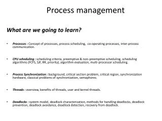
Process management What are we going to learn? • Processes : Concept of processes, process scheduling, co-operating processes, inter-process communication. • CPU scheduling :scheduling criteria, preemptive & non-preemptive scheduling, scheduling algorithms (FCFS, SJF, RR, priority), algorithm evaluation, multi-processor scheduling. • Process Synchronization :background, critical section problem, critical region, synchronization hardware, classical problems of synchronization, semaphores. • Threads : overview, benefits of threads, user and kernel threads. • Deadlocks :system model, deadlock characterization, methods for handling deadlocks, deadlock prevention, deadlock avoidance, deadlock detection, recovery from deadlock.
Processconcept Memory • Process is a dynamic entity • Program in execution • Program code • Contains the text section • Program becomes a process when • executable file is loaded in the memory • Allocation of various resources • Processor, register, memory, file, devices • One program code may create several processes • One user opened several MS Word • Equivalent code/text section • Other resources may vary Disk User program
How to represent a process? • Process is a dynamic entity • Program in execution • Program code • Contains the text section • Program counter (PC) • Values of different registers • Stack pointer (SP) (maintains process stack) • Return address, Function parameters • Program status word (PSW) • General purpose registers • Main Memory allocation • Data section • Variables • Heap • Dynamic allocation of memory during process execution
Process State • As a process executes, it changes state • new: The process is being created • ready: The process is waiting to be assigned to a processor • running: Instructions are being executed • waiting: The process is waiting for some event to occur • terminated: The process has finished execution
Process State diagram Job pool Single processor Multiprogramming As a process executes, it changes state • new: The process is being created • running: Instructions are being executed • waiting: The process is waiting for some event to occur • ready: The process is waiting to be assigned to a processor • terminated: The process has finished execution
Process State diagram Job pool Multitasking/Time sharing As a process executes, it changes state • new: The process is being created • running: Instructions are being executed • waiting: The process is waiting for some event to occur • ready: The process is waiting to be assigned to a processor • terminated: The process has finished execution
Process Control Block (PCB) • Process is represented in the operating system by a Process Control Block Information associated with each process • Process state • Program counter • CPU registers • Accumulator, Index reg., stack pointer, general Purpose reg., Program Status Word (PSW) • CPU scheduling information • Priority info, pointer to scheduling queue • Memory-management information • Memory information of a process • Base register, Limit register, page table, segment table • Accounting information • CPU usage time, Process ID, Time slice • I/O status information • List of open files=> file descriptors • Allocated devices
Process Representation in Linux Represented by the C structure task_structpid t pid; /* process identifier */ long state; /* state of the process */ unsigned int time slice /* scheduling information */ struct task struct *parent; /* this process’s parent */ struct list head children; /* this process’s children */ struct files struct *files; /* list of open files */ structmm_struct *mm; /* address space of this pro */ Doubly linked list
CPU Switch From Process to Process Context switch
Context Switch • When CPU switches to another process, the system must save the state of the old process and load the saved state for the new process via a context switch. • Context of a process represented in the PCB • Context-switch time is overhead; the system does no do useful work while switching • The more complex the OS and the PCB -> longer the context switch • Time dependent on hardware support • Some hardware provides multiple sets of registers per CPU -> multiple contexts loaded at once
Process Scheduling • We have various queues • Single processor system • Only one CPU=> only one running process • Selection of one process from a group of processes • Process scheduling
Process Scheduling • Scheduler • Selects a process from a set of processes • Two kinds of schedulers 1. Long term schedulers, job scheduler • A large number of processes are submitted (more than memory capacity) • Stored in disk • Long term scheduler selects process from job pool and loads in memory 2. Short term scheduler, CPU scheduler • Selects one process among the processes in the memory (ready queue) • Allocates to CPU
Long Term Scheduler CPU scheduler
Scheduling queues • Maintains scheduling queues of processes • Job queue – set of all processes in the system • Ready queue – set of all processes residing in main memory, ready and waiting to execute • Device queues – set of processes waiting for an I/O device • Processes migrate among the various queues
Scheduling queues Job queue Long Term Scheduler Ready queue CPU scheduler Device queue
Ready Queue And Various I/O Device Queues Queues are linked list of PCB’s Device queue Many processes are waiting for disk
Representation of Process Scheduling CPU scheduler selects a process Dispatched (task of Dispatcher) Parent at wait()
Dispatcher • Dispatcher module gives control of the CPU to the process selected by the short-term scheduler; this involves: • switching context • switching to user mode • jumping to the proper location in the user program to restart that program • Dispatch latency – time it takes for the dispatcher to stop one process and start another running
Creation of PCB a.out Shell Create initial PCB Child Shell Exce() Loader (Loads program image in memory) Update PCB Context switch Insert in ready queue Allocate CPU
ISR for context switch Current <- PCB of current process Context_switch() { switch to kernel mode Disable interrupt; Insert(ready_queue, current); Enable Interrupt; next=CPU_Scheduler(ready_queue); Dispatcher(next); } Dispatcher(next) { Save_PCB(current); switch to user mode; Load_PCB(next); [update PC] }
Schedulers • Scheduler • Selects a process from a set • Long-term scheduler(or job scheduler) – selects which processes should be brought into the ready queue • Short-term scheduler(or CPU scheduler) – selects which process should be executed next and allocates CPU • Sometimes the only scheduler in a system
Schedulers: frequency of execution • Short-term scheduler is invoked very frequently (milliseconds) (must be fast) • After a I/O request/ Interrupt • Long-term scheduler is invoked very infrequently (seconds, minutes) (may be slow) • The long-term scheduler controls the degree of multiprogramming • Processes can be described as either: • I/O-bound process– spends more time doing I/O than computations, many short CPU bursts • Ready queue empty • CPU-bound process– spends more time doing computations; few very long CPU bursts • Devices unused • Long term scheduler ensures good process mix of I/O and CPU bound processes.
CPU Scheduling • Describe various CPU-scheduling algorithms • Evaluation criteria for selecting a CPU-scheduling algorithm for a particular system
Basic Concepts • Maximum CPU utilization obtained with multiprogramming • Several processes in memory (ready queue) • When one process requests I/O, some other process gets the CPU • Select (schedule) a process and allocate CPU
Observed properties of Processes • CPU–I/O Burst Cycle • Process execution consists of a cycle of CPU execution and I/O wait • Study the duration of CPU bursts
Histogram of CPU-burst Times Utility of CPU scheduler CPU bound process I/O bound process Large number of short CPU bursts and small number of long CPU bursts
Preemptive and non preemptive • Selects from among the processes in ready queue, and allocates the CPU to one of them • Queue may be ordered in various ways (not necessarily FIFO) • CPU scheduling decisions may take place when a process: 1. Switches from running to waiting state 2. Switches from running to ready state 3. Switches from waiting to ready • Terminates • Scheduling under 1 and 4 is nonpreemptive • All other scheduling is preemptive
Preemptive scheduling Preemptive scheduling Results in cooperative processes Issues: • Consider access to shared data • Process synchronization • Consider preemption while in kernel mode • Updating the ready or device queue • Preempted and running a “ps -el” or “device deiver”
Scheduling Criteria • CPU utilization – keep the CPU as busy as possible • Throughput – # of processes that complete their execution per time unit • Turnaround time – amount of time to execute a particular process • Waiting time – amount of time a process has been waiting in the ready queue • Response time – amount of time it takes from when a request was submitted until the first response is produced, not output (for time-sharing environment)
Scheduling Algorithm Optimization Criteria • Max CPU utilization • Max throughput • Min turnaround time • Min waiting time • Min response time • Mostly optimize the average • Sometimes optimize the minimum or maximum value • Minimize max response time • For interactive system, variance is important • E.g. response time • System must behave in predictable way
Scheduling algorithms • First-Come, First-Served (FCFS) Scheduling • Shortest-Job-First (SJF) Scheduling • Priority Scheduling • Round Robin (RR)
First-Come, First-Served (FCFS) Scheduling • Process that requests CPU first, is allocated the CPU first • Ready queue=>FIFO queue • Non preemptive • Simple to implement • Performance evaluation • Ideally many processes with several CPU and I/O bursts • Here we consider only one CPU burst per process
P1 P2 P3 0 24 27 30 First-Come, First-Served (FCFS) Scheduling ProcessBurst Time P1 24 P2 3 P3 3 • Suppose that the processes arrive in the order: P1 , P2 , P3 The Gantt Chart for the schedule is: • Waiting time for P1 = 0; P2 = 24; P3 = 27 • Average waiting time: (0 + 24 + 27)/3 = 17
P2 P3 P1 0 3 6 30 FCFS Scheduling (Cont.) Suppose that the processes arrive in the order: P2 , P3 , P1 • The Gantt chart for the schedule is: • Waiting time for P1 = 6;P2 = 0; P3 = 3 • Average waiting time: (6 + 0 + 3)/3 = 3 • Much better than previous case • Average waiting time under FCFS heavily depends on process arrival time and burst time • Convoy effect - short process behind long process • Consider one CPU-bound and many I/O-bound processes
Shortest-Job-First (SJF) Scheduling • Associate with each process the length of its next CPU burst • Allocate CPU to a process with the smallest next CPU burst. • Not on the total CPU time • Tie=>FCFS
P3 P2 P4 P1 3 9 16 24 0 Example of SJF ProcessArriva l TimeBurst Time P10.0 6 P2 2.0 8 P34.0 7 P45.0 3 • SJF scheduling chart • Average waiting time = (3 + 16 + 9 + 0) / 4 = 7 Avg waiting time for FCFS?
SJF • SJF is optimal – gives minimum average waiting time for a given set of processes (Proof: home work!) • The difficulty is knowing the length of the next CPU request • Useful for Long term scheduler • Batch system • Could ask the user to estimate • Too low value may result in “time-limit-exceeded error”
P1 P3 P4 P2 P1 0 5 1 10 17 26 Preemptive versionShortest-remaining-time-first • Preemptive version called shortest-remaining-time-first • Concepts of varying arrival times and preemption to the analysis ProcessAarriArrival TimeTBurst Time P10 8 P2 1 4 P32 9 P43 5 • Preemptive SJF Gantt Chart • Average waiting time = [(10-1)+(1-1)+(17-2)+5-3)]/4 = 26/4 = 6.5 msec Avg waiting time for non preemptive?
Determining Length of Next CPU Burst • Estimation of the CPU burst length – should be similar to the previous burst • Then pick process with shortest predicted next CPU burst • Estimation can be done by using the length of previous CPU bursts, using time series analysis • Commonly, α set to ½ Boundary cases α=0, 1
Examples of Exponential Averaging • =0 • n+1 = n • Recent burst time does not count • =1 • n+1 = tn • Only the actual last CPU burst counts • If we expand the formula, we get: n+1 = tn+(1 - ) tn-1+ … +(1 - )j tn-j+ … +(1 - )n +1 0 • Since both and (1 - ) are less than or equal to 1, each successive term has less weight than its predecessor
Priority Scheduling • A priority number (integer) is associated with each process • The CPU is allocated to the process with the highest priority (smallest integer highest priority) • Set priority value • Internal (time limit, memory req., ratio of I/O Vs CPU burst) • External (importance, fund etc) • SJF is priority scheduling where priority is the inverse of predicted next CPU burst time • Two types • Preemptive • Nonpreemptive • Problem Starvation – low priority processes may never execute • Solution Aging – as time progresses increase the priority of the process nice
P1 P5 P3 P4 P2 0 6 1 16 18 19 Example of Priority Scheduling ProcessA arri Burst TimeTPriority P1 10 3 P2 1 1 P32 4 P41 5 P5 5 2 • Priority scheduling Gantt Chart • Average waiting time = 8.2 msec
Round Robin (RR) • Designed for time sharing system • Each process gets a small unit of CPU time (time quantum q), usually 10-100 milliseconds. • After this time has elapsed, the process is preempted and added to the end of the ready queue. • Implementation • Ready queue as FIFO queue • CPU scheduler picks the first process from the ready queue • Sets the timer for 1 time quantum • Invokes despatcher • If CPU burst time < quantum • Process releases CPU • Else Interrupt • Context switch • Add the process at the tail of the ready queue • Select the front process of the ready queue and allocate CPU
P1 P2 P3 P1 P1 P1 P1 P1 0 10 14 18 22 26 30 4 7 Example of RR with Time Quantum = 4 ProcessBurst Time P1 24 P2 3 P3 3 • The Gantt chart is: • Avg waiting time = ((10-4)+4+7)/3=5.66
Round Robin (RR) • Each process has a time quantum T allotted to it • Dispatcher starts process P0, loads a external counter (timer) with counts to count down from T to 0 • When the timer expires, the CPU is interrupted • The ISR invokes the dispatcher • The dispatcher saves the context of P0 • PCB of P0 tells where to save • The dispatcher selects P1 from ready queue • The PCB of P1 tells where the old state, if any, is saved • The dispatcher loads the context of P1 • The dispatcher reloads the counter (timer) with T • The ISR returns, restarting P1 (since P1’s PC is now loaded as part of the new context loaded) • P1 starts running
Round Robin (RR) • If there are n processes in the ready queue and the time quantum is q • then each process gets 1/n of the CPU time in chunks of at most q time units at once. • No process waits more than (n-1)q time units. • Timer interrupts every quantum to schedule next process • Performance depends on time quantum q • q large FIFO • q small Processor sharing (n processes has own CPU running at 1/n speed)
Effect of Time Quantum and Context Switch Time Performance of RR scheduling • No overhead • However, poor response time • Too much overhead! • Slowing the execution time • q must be large with respect to context switch, otherwise overhead is too high • q usually 10ms to 100ms, context switch < 10 microsec