Download
1 / 59
590 likes | 633 Views
The Difference Engine, Charles Babbage Images from Wikipedia (Joe D and Andrew Dunn) Slides courtesy Anselmo Lastra. COMP 740: Computer Architecture and Implementation. Montek Singh Wed, Jan 12, 2011 Lecture 2: Fundamentals and Trends. Quantitative Principles of Computer Design.

E N D
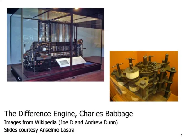
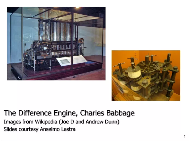
The Difference Engine, Charles Babbage Images from Wikipedia (Joe D and Andrew Dunn) Slides courtesy Anselmo Lastra
COMP 740:Computer Architecture and Implementation Montek Singh Wed, Jan 12, 2011 Lecture 2: Fundamentals and Trends
Quantitative Principles of Computer Design Performance Rate of producing results Throughput Bandwidth Execution time Response time Latency
Topics • Performance • Chips • Trends in • “Bandwidth” (or Throughput) vs. Latency • Power • Cost • Dependability • Measuring Performance
Trends: Moore’s Law Era of the microprocessor. Increases due to transistors and architectural improvements
Performance • Increase by 2002 was 7X faster than would have been due to tech alone • What has slowed the trend? • Note what is really being built • A commodity device! • So cost is very important • Problems • Amount of heat that can be removed economically • Limits to instruction level parallelism • Memory latency
Moore’s Law • Number of transistors on a chip • at the lowest cost/component • It’s not quite clear what it is • Moore’s original paper, doubling yearly • Didn’t make it in 1975 • Often quoted as doubling every 18 months • Sometimes as doubling every two years • Moore’s article worth reading if you haven’t yet
Quick Look: Classes of Computers • Used to be • mainframe, • mini and • micro • Now • Desktop (portable?) • Price/performance, single app, graphics • Server • Reliability, scalability, throughput • Embedded • Not only “toasters”, but also cell phones, etc. • Cost, power, real-time performance
Chip Performance • Based on a number of factors • Feature size (or “technology” or “process”) • Determines transistor & wire density • Used to be measured in microns, now nanometers • Currently: 90 nm, 65 nm, even 45 nm • Die size • Device speed • Note section on wires in HP4 • Thin wires -> more resistance and capacitance • Wire delay scales poorly
ITRS International Technology Roadmap for Semiconductors • http://www.itrs.net/ • An industry consortium • Predicts trends • Take a look at the yearly report on their website
Aside: Ray Kurzweil • Kurzweil: futurist, author • Book in 2005: “The Singularity is Near” • Movie in 2010
Trends • Now let’s look at trends in • “Bandwidth” (Throughput) vs. Latency • Power • Cost • Dependability • Performance
Bandwidth over Latency • Very important to understand section in HP4 on page 15 • What they mean by bandwidth is also processor performance (throughput), maybe memory size, etc • Let’s look at charts
Processor CPU high, Memory low(“Memory Wall”)
Summary • In the time that bandwidth doubles, latency improves by no more than a factor of 1.2 to 1.4 • (and capacity improves faster than bandwidth) • Stated alternatively: • Bandwidth improves by more than the square of the improvement in Latency
Why Less Improvement? • Moore’s Law helps bandwidth • Longer distance for signal to travel, so longer latency • Which offsets faster transistors • Distance limits latency • Speed of light lower bound • Bandwidth sells • Capacity, processor “speed” and benchmark scores • Latency can help bandwidth • Often bandwidth is increased by adding latency • OS introduces latency
Techniques to Ameliorate • Caching • Use capacity (“bandwidth”) to reduce average latency • Replication • Again, leverage capacity • Prediction • Use extra processing transistors to pre-fetch • Maybe also to recompute instead of fetch
Trends • Now let’s look at trends in • “Bandwidth” vs. Latency • Power • Cost • Dependability • Performance
Power • For CMOS chips, traditional dominant energy consumption has been in switching transistors, called dynamic power • For mobile devices, energy is better metric: • For fixed task, slowing clock rate reduces power, not energy • Capacitive load a function of number of transistors connected to output and of technology, which determines capacitance of wires and transistors • Dropping voltage helps both, moved from 5V to 1V • Clock gating
Example • Suppose 15% reduction in voltage results in a 15% reduction in frequency. What is impact on dynamic power?
Trends in Power • Because leakage current flows even when a transistor is off, now static power important too • Leakage current increases in processors with smaller transistor sizes • Increasing the number of transistors increases power even if they are turned off • In 2006, goal for leakage is 25% of total power consumption; high performance designs at 40% • Very low power systems even gate voltage to inactive modules to control loss due to leakage
Trends • Now let’s look at trends in • “Bandwidth” vs. Latency • Power • Cost • Dependability • Performance
Cost of Integrated Circuits Dingwall’s Equation
Explanations Second term in “Dies per wafer” corrects for the rectangular dies near the periphery of round wafers “Die yield” assumes a simple empirical model: defects are randomly distributed over the wafer, and yield is inversely proportional to the complexity of the fabrication process (indicated by a) a=3 for modern processes implies that cost of die is proportional to (Die area)4
Real World Examples “Revised Model Reduces Cost Estimates”, Linley Gwennap, Microprocessor Report 10(4), 25 Mar 1996
Trends • Now let’s look at trends in • “Bandwidth” vs. Latency • Power • Cost • Dependability • Performance
Dependability • When is a system operating properly? • Infrastructure providers now offer Service Level Agreements (SLA) to guarantee that their networking or power service would be dependable • Systems alternate between 2 states of service with respect to an SLA: • Service accomplishment, where the service is delivered as specified in SLA • Service interruption, where the delivered service is different from the SLA • Failure = transition from state 1 to state 2 • Restoration = transition from state 2 to state 1
Definitions Module reliability = measure of continuous service accomplishment (or time to failure) • Two key metrics: • Mean Time To Failure (MTTF) measures Reliability • Failures In Time (FIT) = 1/MTTF, the rate of failures • Traditionally reported as failures per billion hours of operation • Derived metrics: • Mean Time To Repair (MTTR) measures Service Interruption • Mean Time Between Failures (MTBF) = MTTF+MTTR • Module availability measures service as alternate between the 2 states of accomplishment and interruption (number between 0 and 1, e.g. 0.9) • Module availability = MTTF / ( MTTF + MTTR)
Example -- Calculating Reliability • If modules have exponentially distributed lifetimes (age of module does not affect probability of failure), overall failure rate is the sum of failure rates of the modules • Calculate FIT and MTTF for 10 disks (1M hour MTTF per disk), 1 disk controller (0.5M hour MTTF), and 1 power supply (0.2M hour MTTF): Solution next
Solution • If modules have exponentially distributed lifetimes (age of module does not affect probability of failure), overall failure rate is the sum of failure rates of the modules • Calculate FIT and MTTF for 10 disks (1M hour MTTF per disk), 1 disk controller (0.5M hour MTTF), and 1 power supply (0.2M hour MTTF):
Trends • Now let’s look at trends in • “Bandwidth” vs. Latency • Power • Cost • Dependability • Performance
First, What is Performance? • The starting point is universally accepted • “The time required to perform a specified amount of computation is the ultimate measure of computer performance” • How should we summarize (reduce to a single number) the measured execution times (or measured performance values) of several benchmark programs? • Two properties • A single-number performance measure for a set of benchmarks expressed in units of time should be directly proportional to the total (weighted) time consumed by the benchmarks. • A single-number performance measure for a set of benchmarks expressed as a rate should be inversely proportional to the total (weighted) time consumed by the benchmarks. from “Characterizing Computer Performance with a Single Number”, J. E. Smith, CACM, October 1988, pp. 1202-1206
Quantitative Principles of Computer Design • Performance is in units of things per sec • So bigger is better • What if we are primarily concerned with response time? Performance Rate of producing results Throughput Bandwidth Execution time Response time Latency
Performance: What to measure? • What about just MIPS and MFLOPS? • Usually rely on benchmarks vs. real workloads • Older measures were • Kernels or • Small programs designed to mimic real workloads • Whetstone, Dhrystone • http://www.netlib.org/benchmark • Note LINPACK and Top500
MIPS • Machines with different instruction sets? • Programs with different instruction mixes? • Uncorrelated with performance • Marketing metric • “Meaningless Indicator of Processor Speed”
MFLOP/s • Popular in supercomputing community • Often not where time is spent • Not all FP operations are equal • “Normalized” MFLOP/s • Can magnify performance differences • A better algorithm (e.g., with better data reuse) can run faster even with higher FLOP count
Benchmarks • To increase predictability, collections of benchmark applications, called benchmark suites, are popular • SPECCPU: popular desktop benchmark suite • CPU only, split between integer and floating point programs • SPECint2000 has 12 integer, SPECfp2000 has 14 integer pgms • SPECCPU2006 was announced Spring 2006 • SPECSFS (NFS file server) and SPECWeb (WebServer) added as server benchmarks • www.spec.org • Transaction Processing Council measures server performance and cost-performance for databases • TPC-C Complex query for Online Transaction Processing • TPC-H models ad hoc decision support • TPC-W a transactional web benchmark • TPC-App application server and web services benchmark
How to Summarize Performance? • Arithmetic average of execution times?? • But they vary in basic speed, so some would be more important than others in arithmetic average • Could add weights per program, but how to pick weight? • Different companies want different weights for their products • SPECRatio: Normalize execution times to reference computer, yielding a ratio proportional to performance = • time on reference computer / time on computer being rated • Spec uses an older Sun machine as reference
Ratios • If program SPECRatio on Computer A is 1.25 times bigger than Computer B, then • Note that when comparing 2 computers as a ratio, execution times on the reference computer drop out, so choice of reference computer is irrelevant
Geometric Mean • Since ratios, proper mean is geometric mean (SPECRatio unitless, so arithmetic mean meaningless) • Geometric mean of the ratios is the same as the ratio of the geometric means • Ratio of geometric means = Geometric mean of performance ratios choice of reference computer is irrelevant! • These two points make geometric mean of ratios attractive to summarize performance
Different Take • Smith (CACM 1988, see references) takes a different view on means • First let’s look at example