Learning in networks (and other asides)

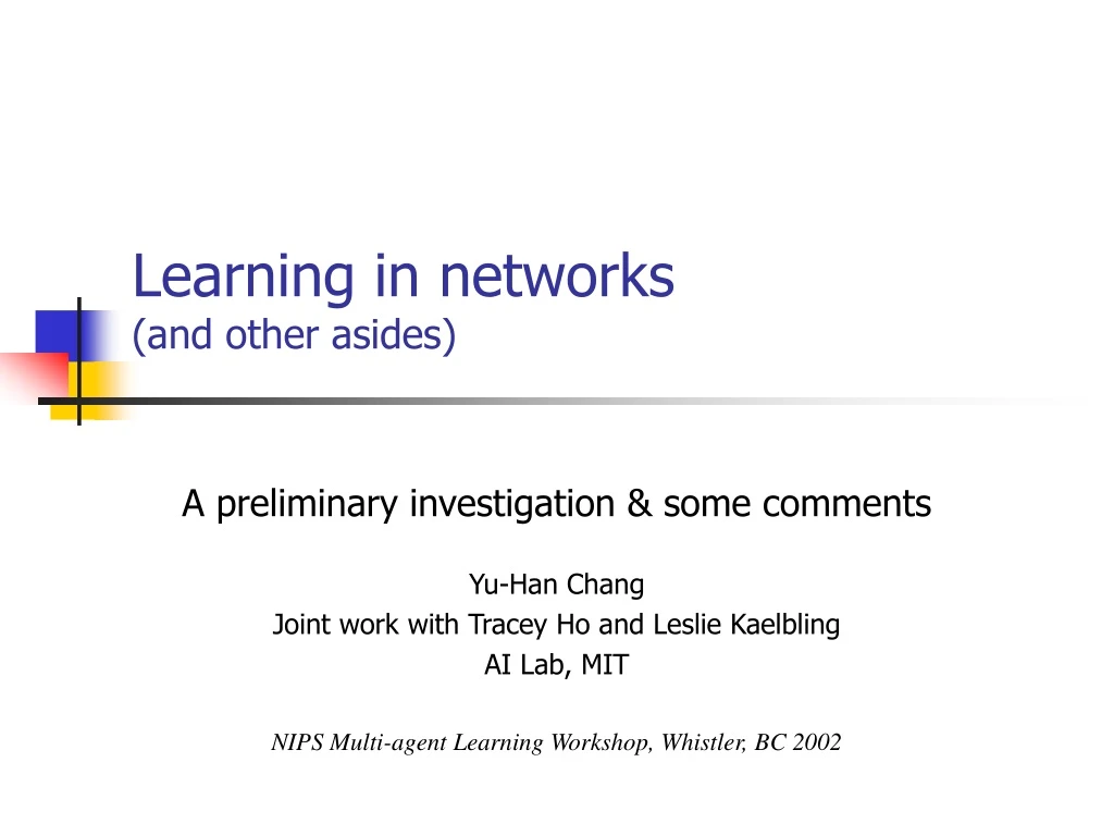
1. Learning in networks(and other asides) A preliminary investigation & some comments Yu-Han Chang Joint work with Tracey Ho and Leslie Kaelbling AI Lab, MIT NIPS Multi-agent Learning Workshop, Whistler, BC 2002

2. Networks: a multi-agent system • Graphical games [Kearns, Ortiz, Guestrin, …] • Real networks, e.g. a LAN [Boyan, Littman, …] • “Mobile ad-hoc networks” [Johnson, Maltz, …]

3. Mobilized ad-hoc networks • Mobile sensors, tracking agents, … • Generally a distributed system that wants to optimize some global reward function

4. Learning • Nash equilibrium is the phrase of the day, but is it a good solution? • Other equilibria, i.e. refinements of NE • Can we do better than Nash Equilibrium? (Game playing approach) • Perhaps we want to just learn some good policy in a distributed manner. Then what? (Distributed problem solving)

5. What are we studying? Learning RL, NDP Stochastic games, Learning in games, … Decision Theory, Planning Game Theory Known world Multiple agents Single-agent

6. Policy Part I: Learning Rewards Observations, Sensations Learning Algorithm World, State Actions

7. Policy Learning to act in the world Other agents (possibly learning) Rewards Observations, Sensations ? Learning Algorithm Environ-ment Actions World

8. A simple example • The problem: Prisoner’s Dilemma • Possible solutions: Space of policies • The solution metric: Nash equilibrium Player 2’s actions World, State Player 1’s actions Rewards

9. That Folk Theorem • For discount factors close to 1, any individually rational payoffs are feasible (and are Nash) in the infinitely repeated game R2 (-2,2) (1,1) R1 safety value (-1,-1) (2,-2)

10. Better policies: Tit-for-Tat • Expand our notion of policies to include maps from past history to actions • Our choice of action now depends on previous choices (i.e. non-stationary) Tit-for-Tat Policy: ( . , Defect ) Defect ( . , Cooperate )  Cooperate history (last period’s play)

11. Types of policies & consequences Stationary:1  At • At best, leads to same outcome as single-shot Nash Equilibrium against rational opponents Reactionary:{ ( ht-1) }  At • Tit for Tat achieves “best” outcome in Prisoners Dilemma Finite Memory: { ( ht-n , … , ht-2 , ht-1) }  At • May be useful against more complex opponents or in more complex games “Algorithmic”: { ( h1 ,h2 , … , ht-2 , ht-1) }  At • Makes use of the entire history of actions as it learns over time

12. Classifying our policy space We can classify our learning algorithm’s potential power by observing the amount of history its policies can use • Stationary: H0 1  At • Reactionary: H1 { ( ht-1) }  At • Behavioral/Finite Memory:Hn { ( ht-n , … , ht-2 , ht-1) }  At • Algorithmic/Infinite Memory:H { ( h1 , h2 , … , ht-2 , ht-1) }  At

13. Classifying our belief space Its also important to quantify our belief space, i.e. our assumptions about what types of policies the opponent is capable of playing • Stationary:B0 • Reactionary:B1 • Behavioral/Finite Memory:Bn • Infinite Memory/Arbitrary:B

14. A Simple Classification

15. A Classification

16. H x B0 : Stationary opponent • Since the opponent is stationary, this case reduces the world to an MDP. Hence we can apply any traditional reinforcement learning methods • Policy hill climber (PHC) [Bowling & Veloso, 02] Estimates the gradient in the action space and follows it towards the local optimum • Fictitious play [Robinson, 51] [Fudenburg & Levine, 95] Plays a stationary best response to the statistical frequency of the opponent’s play • Q-learning (JAL) [Watkins, 89] [Claus & Boutilier, 98] Learns Q-values of states and possibly joint actions

17. A Classification

18. H0 x B : My enemy’s pretty smart • “Bully” [Littman & Stone, 01] Tries to force opponent to conform to the preferred outcome by choosing to play only some part of the game matrix Them: The “Chicken” game (Hawk-Dove) Undesirable Nash Eq. Us:

19. Achieving “perfection” • Can we design a learning algorithm that will perform well in all circumstances? • Prediction • Optimization • But this is not possible!* • [Nachbar, 95] [Binmore, 89] • * Universal consistency (Exp3 [Auer et al, 02], smoothed fictitious play [Fudenburg & Levine, 95]) does provide a way out, but it merely guarantees that we’ll do almost as well as any stationary policy that we could have used

20. A reasonable goal? • Can we design an algorithm in H x Bn or in a subclass of H x Bthat will do well? • Should always try to play a best response to any given opponent strategy • Against a fully rational opponent, should thus learn to play a Nash equilibrium strategy • Should try to guarantee that we’ll never do too badly • One possible approach: given knowledge about the opponent, model its behavior and exploit its weaknesses (play best response) • Let’s start by constructing a player that plays well against PHC players in 2x2 games

21. 2x2 Repeated Matrix Games • We choose row i to play • Opponent chooses column j to play • We receive reward rij , they receive cij

22. Iterated gradient ascent • System dynamics for 2x2 matrix games take one of two forms: Player 2’s probability for Action 1 Player 2’s probability for Action 1 Player 1’s probability for Action 1 Player 1’s probability for Action 1 [Singh Kearns Mansour, 00]

23. Can we do better and actually win? • Singh et al show that we can achieve Nash payoffs • But is this a best response? We can do better… • Exploit while winning • Deceive and bait while losing Them: Matching pennies Us:

24. A winning strategy against PHC 1 If winning play probability 1 for current preferred action in order to maximize rewards while winning If losing play a deceiving policy until we are ready to take advantage of them again 0.5 Probability opponent plays heads 0 1 0.5 Probability we play heads

25. Formally, PHC does: • Keeps and updates Q values: • Updates policy:

26. PHC-Exploiter • Updates policy differently if winning vs. losing: If we are winning: Otherwise, we are losing:

27. PHC-Exploiter • Updates policy differently if winning vs. losing: If Otherwise, we are losing:

28. PHC-Exploiter • Updates policy differently if winning vs. losing: If Otherwise, we are losing:

29. But we don’t have complete information • Estimate opponent’s policy 2at each time period • Estimate opponent’s learning rate 2 t t-2w t-w time w

30. Ideally we’d like to see this: winning losing

31. With our approximations:

32. And indeed we’re doing well. losing winning

33. Knowledge (beliefs) are useful • Using our knowledge about the opponent, we’ve demonstrated one case in which we can achieve better than Nash rewards • In general, we’d like algorithms that can guarantee Nash payoffs against fully rational players but can exploit bounded players (such as a PHC)

34. So what do we want from learning? • Best Response / Adaptive : exploit the opponent’s weaknesses, essentially always try to play a best response • Regret-minimization : we’d like to be able to look back and not regret our actions; we wouldn’t say to ourselves: “Gosh, why didn’t I choose to do that instead…”

35. A next step • Expand the comparison class in universally consistent (regret-minimization) algorithms to include richer spaces of possible strategies • For example, the comparison class could include a best-response player to a PHC • Could also include all t-period strategies

36. Part II • What if we’re cooperating?

37. What if we’re cooperating? • Nash equilibrium is not the most useful concept in cooperative scenarios • We simply want to distributively find the global (perhaps approximately) optimal solution • This happens to be a Nash equilibrium, but its not really the point of NE to address this scenario • Distributed problem solving rather than game playing • May also deal with modeling emergent behaviors

38. Mobilized ad-hoc networks • Ad-hoc networks are limited in connectivity • Mobilized nodes can significantly improve connectivity

39. Network simulator

40. Connectivity bounds • Static ad-hoc networks have loose bounds of the following form: Given n nodes uniformly distributed i.i.d. in a disk of area A, each with range the graph is connected almost surely as n iff n.

41. Connectivity bounds • Allowing mobility can improve our loose bounds to: • Can we achieve this or even do significantly better than this?

42. Many challenges • Routing • Dynamic environment: neighbor nodes moving in and out of range, source and receivers may also be moving • Limited bandwidth: channel allocation, limited buffer sizes • Moving • What is the globally optimal configuration? • What is the globally optimal trajectory of configurations? • Can we learn a good policy using only local knowledge?

43. Routing • Q-routing [Boyan Littman, 93] • Applied simple Q-learning to the static network routing problem under congestion • Actions: Forward packet to a particular neighbor node • States: Current packet’s intended receiver • Reward: Estimated time to arrival at receiver • Performed well by learning to route packets around congested areas • Direct application of Q-routing to the mobile ad-hoc network case • Adaptations to the highly dynamic nature of mobilized ad-hoc networks

44. Movement: An RL approach • What should our actions be? • North, South, East, West, Stay Put • Explore, Maintain connection, Terminate connection, etc. • What should our states be? • Local information about nodes, locations, and paths • Summarized local information • Globally shared statistics • Policy search? Mixture of experts?

45. Macros, options, complex actions • Allow the nodes (agents) to utilize complex actions rather than simple N, S, E, W type movements • Actions might take varying amounts of time • Agents can re-evaluate whether to continue to do the action or not at each time step • If the state hasn’t really changed, then naturally the same action will be chosen again

46. Example action: “plug” • Sniff packets in neighborhood • Identify path (source, receiver pair) with longest average hops • Move to that path • Move along this path until a long hop is encountered • Insert yourself into the path at this point, thereby decreasing the average hop distance

47. Some notion of state • State space could be huge, so we choose certain features to parameterize the state space • Connectivity, average hop distance, … • Actions should change the world state • Exploring will hopefully lead to connectivity, plugging will lead to smaller average hops, …

48. Experimental results

49. Seems to work well

50. Pretty pictures