Download
1 / 23
230 likes | 333 Views
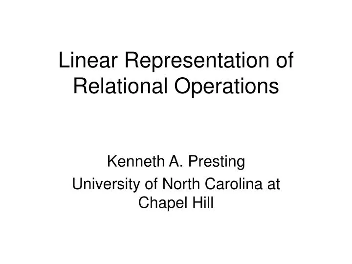
Linear Representation of Relational Operations. Kenneth A. Presting University of North Carolina at Chapel Hill. Relations on a Domain. Domain is an arbitrary set, Ω Relations are subsets of Ω n All examples used today take Ω n as ordered tuples of natural numbers,

E N D
Linear Representation of Relational Operations Kenneth A. Presting University of North Carolina at Chapel Hill
Relations on a Domain • Domain is an arbitrary set, Ω • Relations are subsets of Ωn • All examples used today take Ωn as ordered tuples of natural numbers, Ωn = {(ai)1≤i≤n | ai N } • All definitions and proofs today can extend to arbitrary domains, indexed by ordinals
Graph of a Relation • We want to study relations extensionally, so we begin from the relation’s graph • The graph is the set of tuples, in the context of the n-dimensional space • n-ary relation → set of n-tuples • Examples: x2 + y2 = p → points on a circle, in a plane z = nx + my + b → points in a plane, in 3-space
Hyperplanes and Lines • Take an n-dimensional Cartesian product, Ωn, as an abstract coordinate space. • Then an n-1 dimensional subspace, Ωn-1, is an abstract hyperplane in Ωn. • For each point (a1,…,an-1) in the hyperplaneΩn-1, there is an abstract “perpendicular line,” Ω x {(a1,…,an-1)}
Illustration Graph, Hyperplane, Perpendicular Line, and Slice
Slices of the Graph • Let F(x1,…,xn) be an n-ary relation • Let the plain symbol F denote its graph: F = {(x1,…,xn)| F(x1,…,xn)} • Let a1,…,an-1 be n-1 elements of Ω • Then for each variable xi there is a set Fxi|a1,…,an-1 = { ωΩ | F(a1,…,ai-1,ω,ai,…, an-1} • This set is the xi’s which satisfy F(…xi…) when all the other variables are fixed
The Matrix of Slices • Every n-ary relation defines n set-valued functions on n-1 variables: Fxi(v1,…,vn-1) = { ωΩ | F(v1,…,vi-1,ω,vi,…,vn-1) } • The n-tuple of these functions is called the “matrix of slices” of the relation F
Properties of the Matrix • Each slice is a subset of the domain • Each function Fxi(v1,…,vn-1) : Ωn-1 → 2Ω maps vectors over the domain to subsets of the domain • Application to measure theory
Inverse Map: Matrices to Relations • Two-stage process, one step at a time • Union across columns in each row: RowF(v1,…,vn-1) = n | i<j → ai = vj U { <ai> Ωn | i=j → ai Fxj(v1,…,vn-1) } j=1 | i>j → ai = vj-1 • Union of n-tuples from every row: F = U<vi>Ωn-1 RowF(v1,…,vn-1)
Properties of the Slicing Maps • Map from relations to matrices is injective but not surjective • Inverse map from matrices to relations is surjective but not injective • Not all matrices in pre-image of a relation follow it homomorphically in operations
Boolean Operations on Matrices • Matrices treated as vectors • i.e., Direct Product of Boolean algebras • Component-wise conjunction • Component-wise disjunction • Component-wise complementation
Cylindrical Algebra Operations • Diagonal Elements • Images of diagonal relations, operate by logical conjunction with operand relation • Cylindrifications • Binding a variable with existential quantifier • Substitutions • Exchange of variables in relational expression
The Diagonal Relations • Matrix images of an identity relation, xi = xj • Example. In four dimensions, x2 = x3 maps to:
Axioms for Diagonals • Universal Diagonal • dκκ = 1 • Independence • κ {λ,μ} → cκ dλμ = dλμ • Complementation • κλ→ cκ (dκλ • F) • cκ (dκλ• ~F) = 0
Cylindrical Identity Elements • 1 is the matrix with all components Ω, i.e. the image of a universal relation such as xi=xi • 0 is the matrix with all components Ø, i.e. the image of the empty relation
Diagonal Operations are Boolean • Boolean conjunction of relation matrix with diagonal relation matrix • Example
Substitution is not Boolean • Substitution of variables permutes the slices – not a component-wise operation • Composition of Diagonal with Substitution sκλF = cκ ( dκλ • F ) • If we assume Boolean arithmetic, then standard matrix multiplication suffices
Boolean Matrix Multiplication • Take union down rows, of intersections across columns
Substitution Operators • Square matrices, indexed by all variables in all relations • Substitution operator is the elementary matrix operator for exchange of columns • Example: in a four-dimensional CA, s32 =
Axioms for Cylindrification • Identity • cκ 0 = 0 • Order • F + cκ F = cκ F • Semi-Distributive • cκ (F + cκ G) = cκ F + cκ G • Commutative • cκcλ F = cλcκ F
Instantiation • Take an n-ary relation, F = F(x1,…,xn) • Fix xi = a, that is, consider the n-1-ary relation F|xi=a = F(x1,…,xi-1,a,xi+1,…,xn) • Each column in the matrix of F|xi=a is: Fxj|xi=a(v1,…,vn-2) = F(v1,…,vj-1,xj,vj,…,vi-1,a,vi+1,…,vn)
Cylindrification as Union • Cylindrification affects all slices in every non-maximal column • Each slice in F|xi is a union of slices from instantiations: Fxj|xi(v1,…,vn-2) = U Fxj|xi=a(v1,…,vn-2) aΩ • Component-wise operation
Conclusion • When cylindrification is defined as union of instantiations - • Matrix representations of relations form a cylindrical algebra.