Download
1 / 34
340 likes | 465 Views
C.1.3b - Area & Definite Integrals: An Algebraic Perspective. Calculus - Santowski. Fast Five. (1) 0.25[f(1) + f(1.25) + f(1.5) + f(1.75)] if f(x) = x 2 + x - 1 (2) Illustrate Q1 with a diagram, showing all relevant details. (A) Review.

E N D
C.1.3b - Area & Definite Integrals: An Algebraic Perspective Calculus - Santowski Calculus - Santowski
Fast Five • (1) 0.25[f(1) + f(1.25) + f(1.5) + f(1.75)] if f(x) = x2 + x - 1 • (2) Illustrate Q1 with a diagram, showing all relevant details Calculus - Santowski
(A) Review • We will continue to move onto a second type of integral the definite integral • Last lesson, we estimated the area under a curve by constructing/drawing rectangles under the curve • Today, we will focus on doing the same process, but from an algebraic perspective, using summations Calculus - Santowski
(B) Summations, ∑ • A series is the sum of a sequence (where a sequence is simply a list of numbers) • Ex: the sequence 2,4,6,8,10,12, …..2n has a an associated sum, written as: • The sum 2 + 4 + 6 + 8 + … + 2n can also be written as 2(1+ 2 + 3 + 4 + … + n) or: Calculus - Santowski
(C) Working with Summations • Ex 1. You are given the following series: • List the first 7 terms of each series Calculus - Santowski
(C) Working with Summations • Ex 1I. You are given the following series: • Evaluate each series Calculus - Santowski
(C) Working with Summations • Ex 1. You are given the following series: • List the first 10 terms of each series Calculus - Santowski
(C) Working with Summations • Ex 1. You are given the following series: • Evaluate each series Calculus - Santowski
(B) Summations, ∑ • Here are “sum” important summation formulas: • (I) sum of the natural numbers (1+2+3+4+….n) • (II) sum of squares (1+4+9+16+….+n2) • (III) sum of cubes (1+8+27+64+….n3) Calculus - Santowski
(E) Working With Summations - GDC • Now, to save all the tedious algebra (YEAHH!!!), let’s use the TI-89 to do sums • First, let’s confirm our summation formulas for i, i2 & i3 and get acquainted with the required syntax Calculus - Santowski
(E) Working With Summations - GDC • So let’s revisit our previous example of • And our 4th example of Calculus - Santowski
(F) Applying Summations • So what do we need summations for? • Let’s connect this algebra skill to determining the area under curves ==> after all, we are simply summing areas of individual rectangles to estimate an area under a curve Calculus - Santowski
PART 2 - The Area Problem • Let’s work with a simple quadratic function, f(x) = x2 + 2 and use a specific interval of [0,3] • Now we wish to estimate the area under this curve Calculus - Santowski
(A) The Area Problem – Rectangular Approximation Method (RAM) • To estimate the area under the curve, we will divide the are into simple rectangles as we can easily find the area of rectangles A = l × w • Each rectangle will have a width of x which we calculate as (b – a)/n where b represents the higher bound on the area (i.e. x = 3) and a represents the lower bound on the area (i.e. x = 0) and n represents the number of rectangles we want to construct • The height of each rectangle is then simply calculated using the function equation • Then the total area (as an estimate) is determined as we sum the areas of the numerous rectangles we have created under the curve • AT = A1 + A2 + A3 + ….. + An • We can visualize the process on the next slide Calculus - Santowski
(A) The Area Problem – Rectangular Approximation Method (RRAM) • We have chosen to draw 6 rectangles on the interval [0,3] • A1 = ½ × f(½) = 1.125 • A2 = ½ × f(1) = 1.5 • A3 = ½ × f(1½) = 2.125 • A4 = ½ × f(2) = 3 • A5 = ½ × f(2½) = 4.125 • A6 = ½ × f(3) = 5.5 • AT = 17.375 square units • So our estimate is 17.375 which is obviously an overestimate Calculus - Santowski
(B) Sums & Rectangular Approximation Method (RRAM) • So let’s apply our summation formulas: • Each rectangle’s area is f(xi)x where f(x) = x2 + 2 • x = 0.5 and xi = 0 + xi • Therefore the area of 6 rectangles is given by Calculus - Santowski
(C) The Area Problem – Rectangular Approximation Method (LRAM) • In our previous slide, we used 6 rectangles which were constructed using a “right end point” (realize that both the use of 6 rectangles and the right end point are arbitrary!) in an increasing function like f(x) = x2 + 2 this creates an over-estimate of the area under the curve • So let’s change from the right end point to the left end point and see what happens Calculus - Santowski
(C) The Area Problem – Rectangular Approximation Method (LRAM) • We have chosen to draw 6 rectangles on the interval [0,3] • A1 = ½ × f(0) = 1 • A2 = ½ × f(½) = 1.125 • A3 = ½ × f(1) = 1.5 • A4 = ½ × f(1½) = 2.125 • A5 = ½ × f(2) = 3 • A6 = ½ × f(2½) = 4.125 • AT = 12.875 square units • So our estimate is 12.875 which is obviously an under-estimate Calculus - Santowski
(D) Sums & Rectangular Approximation Method (LRAM) • So let’s apply our summation formulas: • Each rectangle’s area is f(xi)x where f(x) = x2 + 2 • x = 0.5 and xi = 0 + xi • Therefore the area of 6 rectangles is given by: (Notice change in i???) Calculus - Santowski
(E) The Area Problem – Rectangular Approximation Method (MRAM) • So our “left end point” method (called a left hand Riemann sum or LRAM) gives us an underestimate (in this example) • Our “right end point” method (called a right handed Riemann sum or RRAM) gives us an overestimate (in this example) • We can adjust our strategy in a variety of ways one is by adjusting the “end point” why not simply use a “midpoint” in each interval and get a mix of over- and under-estimates? see next slide Calculus - Santowski
(E) The Area Problem – Rectangular Approximation Method (MRAM) • We have chosen to draw 6 rectangles on the interval [0,3] • A1 = ½ × f(¼) = 1.03125 • A2 = ½ × f (¾) = 1.28125 • A3 = ½ × f(1¼) = 1.78125 • A4 = ½ × f(1¾) = 2.53125 • A5 = ½ × f(2¼) = 3.53125 • A6 = ½ × f(2¾) = 4.78125 • AT = 14.9375 square units which is a more accurate estimate (15 is the exact answer) Calculus - Santowski
(F) Sums & Rectangular Approximation Method (MRAM) • So let’s apply our summation formulas: • Each rectangle’s area is f(xi)x where f(x) = x2 + 2 • x = 0.5 and xi = 0.25 + xi • Therefore the area of 6 rectangles is given by: (Notice change in i??? and the xi expression???) Calculus - Santowski
(G) The Area Problem – Expanding our Example • Now back to our left and right Riemann sums and our original example how can we increase the accuracy of our estimate? • We simply increase the number of rectangles that we construct under the curve • Initially we chose 6, now let’s choose a few more … say 12, 60, and 300 …. • But first, we need to generalize our specific formula! Calculus - Santowski
(G) The Area Problem – Expanding our Example • So we have • Now, x = (b-a)/n = (3 - 0)/n = 3/n • And f(xi) = f(a + xi) = f(0 + 3i/n) = f(3i/n) • So, we have to work with the generalized formula Calculus - Santowski
(G) The Area Problem – Expanding our Example • Does this generalized formula work? • Well, test it with n = 6 as before! Calculus - Santowski
(G) The Area Problem – Expanding our Example (RRAM) Calculus - Santowski
(G) The Area Problem – Expanding our Example Calculus - Santowski
(G) The Area Problem – Expanding our Example (LRAM) Calculus - Santowski
(G) The Area Problem – Expanding our Example (LRAM) Calculus - Santowski
(H) The Area Problem - Conclusion • So our exact area seems to be “sandwiched” between 14.95505 and 15.04505 !!! • So, if increasing the number of rectangles increases the accuracy, the question that needs to be asked is ….. how many rectangles should be used??? • The answer is ….. why not use an infinite number of rectangles!! so now we are back into LIMITS!! • So, the exact area between the curve and the x-axis can be determined by evaluating the following limit: Calculus - Santowski
(H) The Area Problem - Conclusion • So let’s verify the example using the GDC and limits: Calculus - Santowski
(I) The Area Problem – Further Examples • (i) Determine the area between the curve f(x) = x3 – 5x2 + 6x + 5 and the x-axis on [0,4] if we (a) construct 20 rectangles or (b) if we want the exact area • (ii) Determine the exact area between the curve f(x) = x2 – 4 and the x-axis on [0,2] if we (a) construct 30 rectangles or (b) if we want the exact area • (iii) Determine the exact area between the curve f(x) = x2 – 2 and the x-axis on [0,2] if we (a) construct 10 rectangles or (b) if we want the exact area Calculus - Santowski
(J) Homework • Homework to reinforce these concepts from this second part of our lesson: • Handout, Stewart, Calculus - A First Course, 1989, Exercise 10.4, p474-5, Q3,4,6a Calculus - Santowski
Internet Links • Calculus I (Math 2413) - Integrals - Area Problem from Paul Dawkins • Integration Concepts from Visual Calculus • Areas and Riemann Sums from P.K. Ving - Calculus I - Problems and Solutions Calculus - Santowski