Download

1 / 34

E N D
Testing a Claim Chapter 11
1.1 Intro • “I can make 80% of my BBall free throws”. To test my claim, you ask me to shoot 20 free throws. I only make 8 and you say “aha! Someone who makes 80% of their free throws would NEVER only make 8/20!” But I say, ‘hey, what if I’m having a bad day, or am injured, or the ball is dead, or the hoop is bent…” Since all of these are possibilities, you say “OK, well I’ll decide how likely your claim is based on the probability that someone who genuinely makes 80% would shoot 8/20 on one trial run” • (In actuality, the probability that someone who makes 80% free throws only hits 8/20 is .0001 or 1/10,000. This is enough to convince you I’m lying!) • This is the basics of hypothesis testing: an outcome that would rarely happen if a claim were true is good evidence that the claim is not true.
Stating a hypothesis • A statistical test starts with a careful statement of the claims we want to compare. Because the reasoning of tests look for evidence against a claim, we start with the claim we seek evidence AGAINST. • This is called our NULL HYPOTHESIS. • The claim about the population we are trying to find evidence FOR is our ALTERNATIVE hypothesis
Example (one-sided) • Attitudes towards school and study habits on a national survey range from 0 to 200. The mean score for US college students is 115 with a standard deviation of 30. Assume normality in this population. A teacher suspects that older students have better attitudes towards school. She gives the survey to a SRS of 25 students. • We seek evidence AGAINST the claim that Mu = 115. • Null: H0: μ= 115 • Alternate: Ha: μ> 115 *Be sure to state the hypothesis in terms of population b/c we are making inference/claims about our pop!
One vs. Two sided hypoth • If the previous example said the teacher thought that seniors had a DIFFERENT attitude towards study habits (but didn’t specify better or worse), we would be doing a two sided hypothesis because the alternate is that μcould be > or < 115. So we state it as: • Ha: μ≠ 115 • **The alternative hypothesis should express the hopes or suspicions we have before we see the data. It is cheating to first look at the data and then frame Ha to fit what the data show!
Conditions for Significance tests • The same 3 conditions from Chapter 10 should be verified before performing a significance test about a population mean or proportion. • 1. SRS • 2. Normality: • For means (data)- population distribution Normal, or large sample size (n>30) or smaller sample with normal histogram/boxplot/probability plot • For proportions- np > 10 and n(1-p) > 10 • 3. Independence (10)(n)< population
Test Statistic • The significance test compares the value of the parameter (true pop mean, as stated in the null) with the calculated sample mean. Values of the sample far from the true parameter give evidence against H0 • To assess how far the sample statistic is from the population parameter, we have to standardize it (to make comparison) • Test statistic = (sample value = mu)/standard deviation of sampling distribution • this is either sigma/square root n or Sx / square root n, depending on if you know sigma or not
Z test • We will focus on the Z test first, which is when we know sigma, so the Z test statistic formula is: • In that last example, lets say the mean (X bar) of the 25 seniors sampled was 125. Our calculated Z would be (125 – 115)/ (30/√25) = 1.67
P-Value • The p value is the probability of getting your observed statistic, assuming the null is true. The smaller your p value, the less likely it is, and the more confident you are in rejecting your claim (the null). • The p value is the area under the curve from your calculated test statistic, to the tail end. • In the previous example, that’s a little less than .1 or 10%.
Statistical Significance • We typically compare the P-value with a fixed P value to make our decision whether or not we the probability (or P-value) is small enough to reject our claim. We set a P value before calculating our observed test statistic and we call this our significance level. • Most commonly we choose .05 as our cutoff point (meaning we need our calculated p value to be less than .05, indicating there is a less than 5% chance of obtaining our result had our original claim been true. • αis the symbol for our chosen significance level we need to beat. So we would say α=.05
Determining significance • If our calculated (or observed) p-value is less than or equal to our alpha level, we say that the data is “statistically significant at level α” • “significant” doesn’t mean important! It just means you are rejecting your null hypothesis • In the previous example, our P value was .1 which is bigger than α=.05, so we would FAIL to reject our null (meaning our sample didn’t provide enough evidence to reject the claim that seniors have the same attitudes as other students) • (or accept the claim that seniors differ significantly)
Typical alpha levels • Just like confidence intervals, our most typical are .1, .05, .01 • It is possible to have results that are significant at the .05 level, but not the .01 level (example: calculated p value = .04) • If significant at .01, significant at .05 and .1 too (example: p = .003)
Final Step: Interpreting results in context • We make our official decision to reject H0 or fail to reject H0 based on whether we “beat” our chosen alpha level (remember to ‘beat’ it means our calculated p-level was smaller) • *warning! In real life, always set alpha level BEFORE analyzing your data!
11.2 Carrying out significance tests • The process is very similar to constructing confidence intervals. Follow the 4 steps on the following slide (sometimes referred to as our “inference toolbox)
Step 1. Hypothesis: Identify the population of interest and the parameter you want to draw conclusions about (usually the mean, mu). State hypothesis (null and alternative, with appropriate symbols) • Step 2: Conditions: Choose the appropriate inference procedure (in this case/chapter, Z test). Verify the conditions for using it (these are the same 3 conditions as before: SRS, Normality, Independence
Step 3: Calculations: If conditions are met, carry out the inference procedure. • Calculate the test statistic • Find the P-value • Step 4: Interpretation: Interpret your results in the context of the problem • Interpret the P-value or make a decision about rejecting H0 using statistical significance • *3C’s Conclusion, Connection and Context!
Example Executives’ blood pressure P. 706 • Director of a company concerned about effects of stress on employees. According to national center for health, the mean blood pressure for males 35 to 44 years of age is 128 and the standard deviation in this population is 15. The director examines the medical records of 72 male executives in this age group and finds that their mean blood pressure is 129.93. Is this evidence that the company’s male execs is different from the national average?
What do we know? • Population: Males 35-44 μ= 128 σ = 15 • Sample: n = 72 = 129.93 • 1. Hypothesis (words and symbols!) • H0: μ= 128 male executives at this company have a mean blood pressure of 128 • Ha: μ≠ 128 male executives at this company have a mean blood pressure that differs from the national mean of 128
Step 2: Conditions • SRS: not told in sample, so we must assume it was an SRS to proceed • Normality: We do not know that the population distribution of blood pressure among male execs is Normally distributed, but the large sample size (n = 72) guarantees that the sampling distribution of the means will be approximately normal by the CLT. • Independence: We must assume that there at least 10x72 =720 middle aged male execs in this large company (b/c this is the population we are making inferences about…not ALL male execs in the world!)
Step 3: Calculations • Test Statistic: we know sigma, so we do a Z test. = (129.93 – 128)/(15/√72) = 1.09 • P-Value: draw a picture NormalCDF(1.09, 1000) =.1379 (this is area in one tail) multiply by 2, p = .2757
Step 4: Interpretation • More than 27% of the time, an SRS of size 72 from the general male population would have a mean blood pressure at least as far from 128 as that of our sample. The observe mean 129.93 is therefore not good evidence that middle aged male execs at this company have blood pressure that differs from the national average. • If we had originally stated we wanted an alpha level of .05, we would say “fail to reject the null at .05 alpha level. Results non-significant”
Confidence intervals and testing for significance • If you wanted to test for significance using a confidence interval, you would construct your interval (as before) and check to see if μfalls in our interval. If it does NOT, then we reject the null and say we have found significant results. • Remember to construct your interval based on the alpha you set. So if you want α = .01, you have to construct a 99% CI etc.
Example • lets do the previous one, but using a CI and a 90% α level. • Construct interval around =129.93 using our σ = 15 129.93 +/- (1.645)( 15/√72) = (127.02, 132.84) Our true population mean μ= 128 does fall in this interval, so we FAIL TO REJECT the null. Results non-significant.
11.3 Uses and abuses of significance tests • Cautions: • Statistical significance is not the same as practical importance. • A few outliers can produce highly significant results (or destroy the significance of otherwise-convincing data). • NOT ROBUST • Beware of multiple analysis (running multiple alpha levels to attain significance etc).
11.4 Using inference to make decisions • Type I vs. Type II error: when we make a decision based on a significance test (reject vs. fail to reject), we hope our decision is correct, but it may in fact be wrong (we really have no way of knowing- if we did, we wouldn’t have done the test in the first place). • Sometimes we get a rare freak sample and reject the null when it’s actually true, or we might fail to reject when it’s truly a false claim.
Example • What if, after doing the study with the male execs and blood pressure, you find out that the 72 people in your sample just came back from a week long spa vacation and were extra relaxed. Had you tested them during a typical work week, their stress levels and blood pressure would have been MUCH higher. • So the fact that we failed to reject the null, when in reality we should have rejected it (had our data been accurate), is a type II error
Which is more serious? Type I or Type II? • Depends on the study. If we’re talking about a drug for example, failing to reject the null might have disastrous consequences!
Error probabilities • While we never can know if we are making a type I or type II error, we can calculate the probability of making an error. • Probability of making a type I error is just alpha! So if your alpha is .05, the probability of rejecting the null when it is in fact true is 5%
Power and Type II error • Power is the probability of correctly rejecting the null. We want power to be high (meaning when we do a test or experiment, our goal is to reject the null and find something interesting, but in the grand scheme that is meaningless if when you reject the null your probability of it being an erroneous rejection is high). • Since making a type II error is the probability of failing to reject the null when you should have rejected, power is the opposite (or converse) probability. • 1 – probability of a type II error.
Continued • Beta βis our symbol for a type II error • power = 1 – β • High power is desirable. Along with 95% CI’s and .05 significance tests, 80% power is desirable. • Many US govt agencies that provide research funds require a the tests to be sufficient to detect important results 80% of the time using a significance test with alpha = .05.
Increasing power • Increase α. A test at the 5% significance level will have a greater chance of rejecting the null than a 1% level because you have a smaller critical value to beat (aka the strength of evidence required for rejection is less). • Increase the sample size. More data provides more info about x bar, so we will have a better chance of distinguishing values of mu. • Decrease sigma (same effect as increasing sample size…more info about x bar). • Improving the measurement process and restricting attention to a subpopulation are two common ways to decrease sigma.
Best advice? • to maximize power, choose as high an alpha level (type I error probability) as you are willing to risk AND as large a sample as you can afford. • You will not compute power or type II error in this course unless one of them is given to you (then you can calculate the other).