Summary of introduced statistical terms and concepts

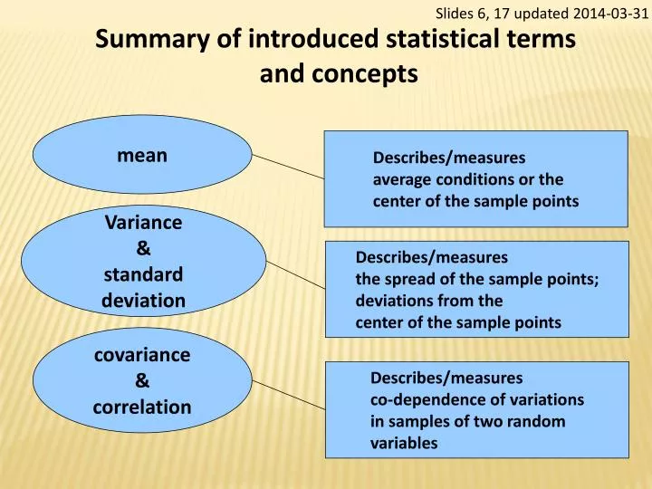
1. Slides 6, 17 updated 2014-03-31 Summary of introduced statistical terms and concepts mean Describes/measures average conditions or the center of the sample points Variance & standard deviation Describes/measures the spread of the sample points; deviations from the center of the sample points covariance & correlation Describes/measures co-dependence of variations in samples of two random variables

2. Summary of introduced statistical terms and concepts Calculated mean values: unbound, any real number (check your values: it must be within the minimum and maximum of the sample data) mean Variance & standard deviation Variance: values are > or = 0 Standard deviation: > or = 0 (check your values: standard deviation should be less than the minimum-maximum sample range |max(x)-min(x)|) covariance & correlation Covariance: any real number Correlation: between -1 and +1 (check your values: correlation should never exceed the range from -1 to 1]

3. Linear function: y= bx +a The value of y depends on the value of x Δy = b*Δx Δx Note: I corrected the notation of the equation, please check your notes b is the slope, a is the constant the intercept value. R-script class14.R was updated (2014-03-25 4:30pm)

4. Linear function y= bx +a The value of y depends on the value of x b= Δy/Δx =2 Δy = b*Δx Δx a=-1

5. Linear function y= bx +a The value of y depends on the value of x value of y does not depend on x a= Δy/Δx =2 y= 0x + a= a

6. Note: updated slide to define y with random error

7. ?

8. How to estimate the best fitting line?

9. How to estimate the best fitting line? Mathematically we formulate this as a minimization problem: Minimize the distance of the data points from the linear regression line.

10. How to estimate the best fitting line? The deviations from the deterministic model line are interpreted as random errors (following a Gaussian distribution) Sum of Squared Errors (SSE)

11. How to estimate the best fitting line? Sum of Squared Errors (SSE) Intercept Slope

12. How to estimate the best fitting line? Sum of Squared Errors (SSE) Sample mean of x and y ^ ^ ^ Note: Many textbooks and statisticians would prefer to distinguish the estimated values from the actual true (but unknown) parameter values using a different symbol. Or they use Greek letters for the true values, and Latin letters for the estimates.

13. 1 n 1 n How to estimate the best fitting line? Sum of Squared Errors (SSE) COV(x,y) b= VAR(x)

14. 1 n 1 n How to estimate the best fitting line? Sum of Squared Errors (SSE) Slope of the regression line: Correlation coefficient * standard deviation (y) / standard deviation (x)

15. How to estimate the best fitting line? Estimated Regression line Linear relationship with errors: y= bx +a + ε The value of y depends on the value of x plus a random error

16. Class exercises: download script class14.R: source(“class14.R”) (1) change the linear parameters to have steeper, or more flat slopes. (2) change the slope to negative (from top left to bottom right) (3) observe how the correlation coefficient changes (4) change the error variance and observe how it affects the correlation and fitting of the line (5) watch in case, where does the line intersect with the y-axis (6) change the intercept parameter (intersection with the y-axis). What is the effect on the correlation? (7) find a way to change the sample size of the scatter points and repeat your (1)-(6) (8) set the slope parameter closer to 0 and eventually to 0 change the variance of the errors. What happens to correlation?

17. Note: In R-scripts the variable names have a slightly different notation: As you can see in class14.R we use ‘yobs’ for the variable y containing the random error ‘e’. The estimator for the slope ‘bfit’ is calculated by using for the correlation coefficient ‘cor(x,yobs)’ and the standard deviation ‘sd(yobs)’ and ‘sd(x)’ The equation on slide 14 includes the error