Download

1 / 47
490 likes | 818 Views
A Randomized Linear-Time Algorithm to Find Minimum Spanning Trees. David R. Karger Philip N. Klein Robert E. Tarjan. Talk Outline. Objective & related work from literatures Intuition Definitions Algorithm Proof & Analysis Conclusion and future work. Objective.

E N D
A Randomized Linear-Time Algorithm to Find Minimum Spanning Trees David R. Karger Philip N. Klein Robert E. Tarjan
Talk Outline • Objective & related work from literatures • Intuition • Definitions • Algorithm • Proof & Analysis • Conclusion and future work
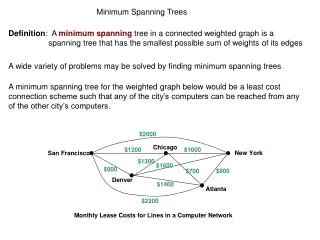
Objective • A minimum spanning tree is a tree formed from a subset of the edges in a given undirected graph, with two properties: 1. it spans the graph, i.e., it includes every vertex in the graph, and 2. it is a minimum, i.e., the total weight of all the edges is as low as possible. Find a minimum spanning tree for a graph by linear time with very high probability!!
Related Work • Boruvka 1926, textbook algorithms – • Yao 1975 – • Cheriton and Tarjan 1976 – • Fredman and Tarjan 1987 – • Gabow 1986 – • Chazelle 1995 – Deterministic results! How about the randomized one??
Intuition • Cycle Property • Cut Property • Randomization
Intuition For any cycle C in a graph, the heaviest edge in C does not apper in the minimum spanning tree.
Heaviest edge Cycle Property
Cycle Property • For any graph, find all possible cycles and remove the heaviest edge from each cycle. Then we can get a minimum spanning tree?? How about the time complexity? How to detect the cycles in the graph??
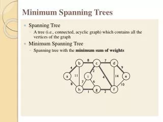
Cut Property For any proper nonempty subset X of the vertices, the lightest edge with exactly one endpoint in X belongs to the minimum spanning tree.
Boruvka Algorithm • For each vertex, select the minimum-weight edge incident to the vertex. Contract all the selected edges, replacing by a single vertex each connected component defined by the selected edges and deleting all resulting isolated vertices, loops (edges both of whose endpoints are the same), and all but the lowest-weight edge among each set of multiple edges. O(m log n)
Randomization How the randomization can help us to achieve our goal? Boruvka + Cycle Property + Randomization = Linear time with very high probability
Definition • Let G be a graph with weighted edges. w(x, y) : the weight of edge {x, y} • If F is a forest of a subgraph in G, F(x, y) : the path (if any) connecting x and y in F, : the maximum weight of an edge on F(x, y), with the convention that if x and y are not connected in F.
Definition • F-heavy Otherwise, {x, y} is F-light.
F-heavy & F-light F-heavy F-light
F-heavy & F-light • Note that the edges of F are all F-light. For any forest F, no F-heavy edge can be in the minimum spanning forest of G. Cycle Property!!
Recursive function call: Input: A undirected graph Output: A minimum spanning forest Time: for the worst case O(m) with very high probability Algorithm
Algorithm • Step 1. Apply two successive Boruvka steps to the graph, thereby reducing the number of vertices by at least a factor of four.
Algorithm • Step 2. In the contracted graph, choose a subgraph H by selecting each edge independently with probability 1/2. Apply the algorithm recursively to H, producing a minimum spanning forest F of H. Find all the F-heavy edges (both those in H and those not in H) and delete them.
Algorithm Back to analysis
Algorithm • Step 3. Apply the algorithm recursively to the remaining graph to compute a spanning forest . Return those edges contracted in Step 1 together with the edges of .
Algorithm Back to analysis
Algorithm F - light Those not in H F - heavy Edges of H
Analysis • Correctness? • Worst-case time complexity? • Expected time complexity?
Correctness • Completeness By the cut property, every edge contracted during Step 1 is in the minimum spanning forest. Hence the remaining edges of the minimum spanning forest of the original graph form a minimum spanning forest of the contracted graph.
Correctness • Soundness By the cycle property, the edges deleted in Step 2 do not belong to minimum spanning forest. By the inductive hypothesis, the minimum spanning forest of the remaining graph is correctly determined in recursive call of Step 3.
Worst-case time complexity • The worst-case running time of the mini-spanning forest algorithm is , the same as the bound for Boruvka’s algorithm. Count the total number of edges. Step 1 reduces the size to ¼ as its original. A subproblem at depth d contains at most edges. Summing all subproblems gives an bound on the total number of edges.
Parent Left Right Worst-case time complexity • Parent: E(G) • Left child: E(H) • Right child: Number of edges in next recursion level = E(G*) + E(F) = E(G) – V(G)/2 + V(G)/4
Worst-case time complexity m edges
Worst-case time complexity • The total time spent in Steps 1-3 is linear in the number of edges: Step 1 is just two steps of Boruvka’s algorithm. Step 2 takes linear time using the modified Dixon-Rauch-Tarjan verification algorithm. - F-heavy edges of G can be computed in time linear in the number of edges of G.
Analysis • Given graph G with n vertices and m edges • After one Boruvka step, Boruvka step forms connected components and replaces each by single vertex. Since each component connects more than 2 edges, there are at most n/2 vertices remained. • For component with k vertices, exactly k – 1 edges are removed. Thus the edges removed is at leastwhere is set of connected components. Since there is at most n/2 components, there is at least n/2 edges removed.
Analysis • Given F = MST(H), for (x, y) in H • If (x, y) is in F, (x, y) is F-light • If (x, y) is not in F, assume (x, y) is F-light, the heaviest edge in cycle P (x, y) would be on P, and is belong to no MST according to cycle property. This causes contradiction, thus (x, y) is F-heavy. • Thus, each F-light edge in H is also in F, and vice versa.
Analysis According to the distribution of edges used by H and G', edges of F are used twice by calling MST(H) and MST(G').
Analysis The binary tree represents the recursive invocation of MST: Left child represents invocation of MST(H). Right child represents invocation of MST(G'). Since 2 Borůvka step are performed before invocation of MST(H) and MST(G'), number of vertices is reduced in factor of 4. Thus, the height of invocation is at most log4n.
Analysis - Worst Case • Given graph G with m edges and n vertices • After 2 Borůvka steps, at most n/4 vertices and m – n /2 edges remain for G*. This is true also for H and G' which are subgraph of G*. • Since F = MST(H), F has at most vH – 1 edges, and thus less than n/4. • According to the edge distribution,eH + eG' eG* + eF m – n/2 + vH m – n/2 + n/4 mThus, the number of edges in subproblems is less than original’s.
Analysis - Worst Case • Since total edge number of subproblems at the same depth is bound by m, and the depth is at most log4n, the overall edge number is at most m log4n. • Since vertex number for submproblem at depth d is at most n/4d, the edge is at most (n/4d)2. Overall edge number is also bound by • Since running time of the algorithm is proportional to edge number, we could give time complexity as O(min{n2, m log n})
Analysis – Average Case Here, we analyze the average case by partitioning the invocations as “left paths” (red paths above). After reckoning edges of subproblems along each “left path”, sum them up and we will get the overall estimate.
Analysis – Average Case • For G* with k edges, after sampling with 1/2 probability for each edge, E[eH] = k/2.Since G* G, we have E[eG*] E(eG) and E[eH] = E[eG*]/2 E[eG]/2. • Along the left path with starting E[eG] = k, the expected value of total edges is
Analysis – Average Case Given vG*= n, F = MST(H) where H G* • For each F-light edge, there is 1/2 probability of being sampled into H. • Since each F-light edge in H is also in F and F includes no edges not in H, the chance that an F-light is in F is also 1/2. • For edge e with weight heavier than the lightest of F is never F-light since there would be cycle with e as heaviest edge. • Thus, the heaviest F-light edge is always in F. Given eF=k, eG' is the number trials before k successes (selected into H), and it forms a negative binomial distribution.
Analysis – Average Case Given vG*= n, F = MST(H) where H G* • For eF = k, eG' is of negative binomial distribution with parameter 1/2 and k. Thus E[eG'] = k/(½) = 2k. • Summing all cases, we get
Analysis – Average Case • For all right subproblems, expected sum of edges is at most • For each left path, the expected total number of edges is twice of the leading subproblem, which is root or right child. So the overall expected value is at most 2(m + n). • Since running time is proportional to overall edge number, so its expected value is O(m) = O(m + n).
Analysis – Probability of Linearity Chernoff Bound: Given xi as i.d.d. random variables and 0< i n, and X is the sum of all xi, for t > 0, we have Thus, the probability that less than s successes (each with cance p) within k trail is
Analysis – Probability of Linearity • Given a path with leading problem G, eG = k • For each edge in G, it has 1/2 less chance to be kept in next subproblem. and each edge-keep contributes 1 to the total edge number. The path ends when the k-th edge-move occurs. • The probability there are 3k more total edges is probability there are k less edge-remove in k+3k trail. According to Chernoff bound, the probability is exp(-(k)).
Analysis – Probability of Linearity • Given vG* = n'. For each edge in G', it has 1/2 chance to be in F. Since eF = n' – 1, the probability that eG' > 3n' is probability there are n' - 1 less F edge in 3k trail. According to Chernoff bound, the probability is exp(-(n')). • There is at most n/2 total vertices in all G*. If we take all the trail as a whole, the probability that there are more than 3n/2 edges in all right subproblem is exp(-(n)).
Analysis – Probability of Linearity Combined with previous two analysis, there is at least probability as below that total edges never exceeds 3(m+3n/2), where is the set of all right problems: Thus, the probability that time complexity is O(m) is1 – exp((m)).