Download
1 / 12
150 likes | 371 Views
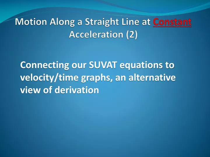
Motion Along a Straight Line at Constant Acceleration (2). Connecting our SUVAT equations to velocity/time graphs, an alternative view of derivation. Learning Objectives :. To revise distance/time and speed/time graphs if necessary.

E N D
Motion Along a Straight Line at Constant Acceleration (2) Connecting our SUVAT equations to velocity/time graphs, an alternative view of derivation
Learning Objectives : To revise distance/time and speed/time graphs if necessary. To show a connection between the SUVAT equations & velocity/time graphs To work through lots more examples of using the SUVAT equations Book Reference : Pages 112-118
Consider some generalised motion, starting with an initial velocity u, accelerating with acceleration a for a period t ending with a final velocity v v a δv Velocity / ms-1 δt u Note δ means small change in time / s t
From our existing knowledge of velocity/time graphs we know that acceleration is given by the gradient of the line: a = δv δt So change in velocity, δv = aδt. So starting at u & after acceleration a for t seconds v = u + at (SUVAT 1) Note δ means small change in
Also from our existing knowledge of velocity/time graphs we know that the distance travelled is the total area under the graph v a v - u Velocity / ms-1 u time / s t
Considering the areas: For the rectangle : area = ut For the triangle : area = ½ base x height area = ½ t (v – u) Total area = ut + ½ t (v – u) 2s = 2ut + t(v – u) s = (u + v)t(SUVAT 2) 2
An alternative view: We are actually trying to find the area of a trapezium which is:- Half the sum of the parallel sides x the distance between the parallel sides ½(u + v) t s = (u + v)t(SUVAT 2) 2
Considering the distance, (area under the graph) this time without v v a v - u Velocity / ms-1 u time / s t Total area = rectangle + triangle s = ut + ½(v – u) t
As before remove our dependence upon v by substituting for it from SUVAT 1 v = u + at s = ut + ½((u + at) – u) t s = ut + ½at2 (SUVAT 3)
Considering the distance, (area under the graph) this time without t v a v - u Velocity / ms-1 u time / s t Total area = rectangle + triangle s = ( u + v )t 2
As before remove our dependence upon t by substituting for it from SUVAT 1 v = u + at t = v – u a s = ( u + v )t 2 s = (u + v) (v – u ) 2a 2as = uv + v2 – uv – u2 v2 = u2 + 2as (SUVAT 4)
S.U.V.A.T Equations Summary (again) v = u + at (1) s = (u + v)t (2) 2 s = ut + ½at2 (3) v2 = u2 + 2as (4)