Download
1 / 29
290 likes | 367 Views
This study presents a novel approach to deforming text in 2D and 3D spaces, utilizing control polygons and surface mapping techniques. The algorithm ensures smooth deformation while preserving text geometry. The process involves subdividing surfaces, distributing text lines, and composing 3D text using Bezier surfaces. By adhering to these methods, intricate text layouts can be achieved with aesthetic appeal.

E N D
Artistic Surface Rendering Using Layout Of Text Tatiana Surazhsky Gershon Elber Technion, Israel Institute of Technology
Background Figure 1: • A deformation of the letter `E' using bending of a base line (thick). • The original character is shown in (a). • Character deformation using mapping of the control polygons is shown in (b). • The deformation of the symbol using the algorithm we adopt here is shown in (c). Base lines are shown thick.
Smooth Deformation of Text in the Plane (1/3) • Consider a text string that has been created with the aid of an outline font. • The geometry of the text is prescribed via a set of linear and cubic Bezier curve segments {Ci(t)}i. • The Bezier curves are defined via a finite number of control points (two in the linear case, and four in the cubic case).
Smooth Deformation of Text in the Plane (2/3) • we first define a planar deformation surface S(u, v) as a mapping from R2 ->R2. • The text to be deformed, {Ci(t)}i, is assumed to be contained in the parametric domain of S(u, v). • S(u, v) is then composed with one curve segment, , at a time. • again assuming all the geometry of the original symbols lie in the parametric domain of the surface S(u, v).
Smooth Deformation of Text in the Plane (3/3) • Figure 2: Two linear and parallel edges of a symbol with a base line (thick) are shown in (a). The deformed base line with the mapped end control points and edges, is shown in (b). The straight lines intersect each other in (b). Moreover, part of the symbol even expand below the base line. Note that the lengths of the dashed lines, h1and h2, (that are normal to the base line) have not been modified.
Text Deformation in Three Dimensions (1/2) • Let S(u, v) be a general B-spline surface. • We now review the algorithm that maps the linear/cubic Bezier geometry, {Ci(t)}i, of the given text onto a general B-spline surface, S(u, v).
Text Deformation in Three Dimensions (2/2) Figure 3: • Planar examples of text deformation. An example of a text layout over the base curve (u) is shown in (a). • In (b), a text deformation guided by a shaping curve (v) is presented. • In this work, we are interested in placing text on a given three dimensional free-form parametric surface. Thus, S(u, v) is assumed to be a general three dimensional free-form surface.
The Surface Subdivision Stage (1/5) • As a first step, S(u, v) is subdivided in the v direction into several strips, the number of which is equal to the number of desired lines of text. • Typically, the field of the parameterization is not uniform along S(u, v). • We seek a distribution of the lines of text on S(u, v) that is fair.
The Surface Subdivision Stage (2/5) • Assume uminand umaxare the minimal and the maximal values of the u parameter in the parametric domain of S(u, v), while vminand vmaxare the bounds of the parameter v. • Calculate the velocity vector field dS(u,v)/dv , and consider it at = (umin+umax)/2 for all v and while subdividing the surface. • For a given number of lines of text, N, we approximate the value of the parameter vifor the bottom cut of the i-th strip so that the following holds: Equation (4.1)
The Surface Subdivision Stage (4/5) • The input text is split into the selected number of lines, so that all the lines would have a length of text that is proportional to the arc-length of that line on the surface. • This process is conducted by computing the length of the entire body of text in relations to the accumulated lengths of all the base lines of surface strips Sj(u, vj) as derived using Equation (4.1).
The Surface Subdivision Stage (5/5) • We strive to break the input text into lines in such a way that the following relation holds: where Ljis the length of the text that is assigned to the j-th surface strip.
Composing 3D Text (1/4) • The B-spline surface representing the j-th strip, Sj(u, v) is first converted into a set of Bezier surfaces by subdividing Sj(u, v) at all its internal knots, ukor vl. • Further, all the Bezier curves are similarly subdivided at the internal knots of ukand vl, solving for the following:
Composing 3D Text (2/4) Figure 5: • The letter 'A' is shown in the parameter space of the surface strip Sj(u, v). • The surface as well as the curve are subdivided at all the interior knots, ukor vl, of Sj(u, v).
Composing 3D Text (3/4) • The deformation is completed by composing the subdivided segments of the Bezier curves with the corresponding subdivided Bezier patches. • Let C(t) = (u(t), v(t)) be a Bezier curve such that u(t), v(t)(0, …,1); 8t and let S be a Bezier surface. where is the i-th Bezier basis function of degree n and Pijare the control points of S.
Composing 3D Text (4/4) • Assuming one can compute and represent the composition as a curve, the curve S(u(t), v(t)) is also representable because it involves sums and products of polynomial terms only, which is polynomial. which is again reduced to sums and products of polynomial terms only.
Shading Computation (1/3) • The text symbols must be properly shaded, taking into account the local shading information of the three dimensional surface. • Emulating this traditional rendering process, we evaluate a single intensity level I for each visible symbol. • The magnitude of I directly controls the width of the symbol.
Shading Computation (2/3) • The cosine shader is one of the most commonly used in computer graphics: • (u; v) are the coordinates of the center of the bounding box of the symbol in the parametric domain of S(u; v), • ωprovides some bias, • L is the unit vector toward the light source, • V stands for the unit vector toward the viewer, • R is the direction of the reflected light, • Ia; Idand Isare the coefficients for the ambient, diffuse and specular components of the illumination. where
Shading Computation (3/3) • Two examples of such additional shaders are a silhouette enhancement shaderand a distance dependent shader. where Is(u, v) is a shader that enhances silhouette areas and Id(u, v) is a distance dependent shader, ω provides bias control as before and ris a decay factor.
Surface Singularities (1/2) • This singularity pose difficulties only at the shading computation stages, a problem that is shared by all surface rendering schemes. • One can approximate the normal at non regular locations, using near by regular locations.
Surface Singularities (2/2) • Other potential difficulties might stem from surfaces of varying arc-length along isoparametric curves and/or surfaces of varying distance between isoparametric curves. • Varying arc-length along isoparametric curves is taken care of by the proper placement of the symbols along the curve (See Equation 4.2)).
Result Figure 7: • A standard cosine shader (Ic, see Equation (4.6)) applied to the model of the Utah teapot. The illumination intensity defines the width of the outline of each symbol. In (a), • the widest parts correspond to the highest intensity levels, while in (b), the lowest intensity levels are associated with the minimal outline width.
Result Figure 8: • An example of a rendering with a shader that enhances silhouette areas (Is, see Equation (4.8)). • (b) presents the enlarged square region of (a).
Result Figure 9: • Examples of the silhouette shader (Is, see Equation (4.8)) application on a pawn (a), • the distance dependent shader (Id, see Equation (4.9)) application on a glass (b).
Result Figure 10: • Examples of the color enhanced cosine shader application on a Utah teapot on (a) and (b) , • a pawn (c). (b) presents the enlarged square region of (a). The specular component adds the red color to otherwise blue surfaces.
Result Table 1: • Running times (AMD Athlon 1.2GHz running Windows 2000) for the given examples.