Download
1 / 6
60 likes | 211 Views
Dilute Liquid Solutions SVNA 10.4,12.1.

E N D
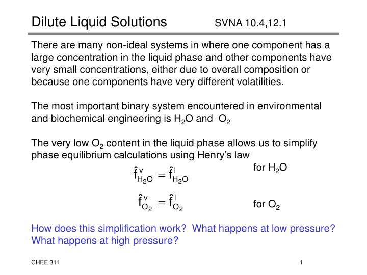
Dilute Liquid Solutions SVNA 10.4,12.1 • There are many non-ideal systems in where one component has a large concentration in the liquid phase and other components have very small concentrations, either due to overall composition or because one components have very different volatilities. The most important binary system encountered in environmental and biochemical engineering is H2O and O2 • The very low O2 content in the liquid phase allows us to simplify phase equilibrium calculations using Henry’s law • for H2O • for O2 • How does this simplification work? What happens at low pressure? What happens at high pressure?
Rigorous Treatment of Liquid Mixture Fugacity • Shown is a plot of the mixture fugacities of MEK (1) and Toluene (2) at 50°C as a function of liquid composition • For component 1, MEK: • For component 2, Toluene: • What happens when we have nearly pure 1 in the liquid? What if we had when we had nearly pure 2 in the liquid? What about at low P?
Dilute Liquid Solution Approximations • This figure shows the fugacity of component 1 in a liquid mixture. The plot is linear at both ends • The Lewis-Randall rule applies when the solution is nearly pure 1: • x11: 1 1, f1l f1lx1 • When component 1 is present in very small amounts (x1 < 0.02), its mixture fugacity can be approximated by a different linear relationship • x10: f1l k1x1 • What are the units of k1?
Dilute Solution Simplifications: Nearly pure component • For nearly pure component (1) of a dilute solution, we can apply the Lewis-Randall rule: • The equilibrium relationship for the nearly pure component (such as H2O (1) in the water-oxygen system) becomes: • or, • or, • for situations where x1>0.98)
Dilute Solution Simplifications: Minor Component • For the minor component (2) of a dilute liquid solution, we use the Henry’s constant, k2,where k2 is the slope of f2l vs x2 curve when x2 0. • Henry’s constants are tabulated for specific systems at a given temperature. • The equilibrium relationship for the minor component (such as O2 in the water-oxygen system) becomes: • where the Henry’s constant, k2 is that of oxygen in water at the temperature of interest. • What happens at low P? How is k2 related to 2 ?