Download
1 / 30
300 likes | 412 Views
Graphs. Storage, Definitions, Coloring, And Traversals. Graphs. Definition (undirected, unweighted ): A Graph G, consists of a set of vertices, V a set of edges, E where each edge is associated with a pair of vertices. We write: G = (V, E). A labeled simple graph:

E N D
Graphs Storage, Definitions, Coloring, And Traversals
Graphs • Definition (undirected, unweighted): • A Graph G, consists of • a set of vertices, V • a set of edges, E • where each edge is associated with a pair of vertices. • We write: G = (V, E) A labeled simple graph: Vertex set V = {1, 2, 3, 4, 5, 6} Edge set E = {{1,2}, {1,5}, {2,3}, {2,5}, {3,4}, {4,5}, {4,6}}.
Graphs • Directed Graph: • Same as above, but where each edge is associated with an ordered pair of vertices. A labeled simple graph: Vertex set V = {2,3,5,7,8,9,10,11} Edge set E = {{3,8}, {3,10}, {5,11}, {7,8}, {7,11}, {8,9}, {11,2},{11,9},{11,10}}.
Graphs • Weighted Graph: • Same as above, but where each edge also has an associated real number with it, known as the edge weight. A labeled weighted graph: Vertex set V = {1,2,3,4,5}
Data Structures to Store Graphs • Edge List Structure • Each vertex object contains a label for that vertex. • Each edge object contains a label for that edge, as well as two references: • one to the starting vertex and one to the ending vertex of that edge. • (In an undirected graph the designation of starting and ending is unnecessary.) Surprisingly, if you implement these two lists with doubly linked lists, our performance for many operations is quite reasonable: • Accessing information about the graph such as its size, number of vertices etc. can be done in constant time by keeping counters in the data structure. • One can loop through all vertices and edges in O(V) or O(E) time, respectively. • Insertion of edges and vertices can be done in O(1) time, assuming you already have access to the two vertices you are connecting with an edge. • Access to edges incident to a vertex takes O(E) time, since all edges have to be inspected.
Data Structures to Store Graphs • Adjacency Matrix Structure • Certain operations are slow using just an adjacency list because one does not have quick access to incident edges of a vertex. • We can add to the Adjacency List structure: • a list of each edge that is incident to a vertex stored at that vertex. • This gives the direct access to incident edges that speeds up many algorithms. • eg. In Dijkstra's we always update estimates by looking at each edge incident to a particular vertex.)
Data Structures to Store Graphs • Adjacency Matrix • The standard adjacency matrix stores a matrix as a 2-D array with each slot in A[i][j] being a 1 if there is an edge from vertex i to vertex j, or storing a 0 otherwise. • Can have a more O-O design: • Each entry in the array is null if no edge is connecting those vertices, or an Edge object that stores all necessary information about the edge. • Although these are very easy to work with mathematically, they are more inefficient than Adjacency lists for several tasks. For example, you must scan all vertices to find all the edges incident to a vertex. • In a relatively sparse graph, using an adjacency matrix would be very inefficient running Dijkstra's algorithm, for example.
Graph Definitions – types of Graphs • A complete undirected unweighted graph • is one where there is an edge connecting all possible pairs of vertices in a graph. The complete graph with n vertices is denoted as Kn. • A graph is bipartite • if there exists a way to partition the set of vertices V, in the graph into two sets V1 and V2 • where V1 V2 = V and V1 V2 = , such that each edge in E contains one vertex from V1 and the other vertex from V2.
Graph Definitions – types of graphs • Complete bipartite graph • A complete bipartite graph on m and n vertices is denoted by Km,n and consists of m+n vertices, with each of the first m vertices is connected to all of the other n vertices, and no other vertices.
Graph Definitions – graph terms • A path • A path of length n from vertex v0 to vertex vn is an alternating sequence of n+1 vertices and n edges beginning with vertex v0 and ending with vertex vn in which edge eiis incident upon vertices vi-1 and vi. • (The order in which these are connected matters for a path in a directed graph in the natural way.) • A connected graph • A connected graph is one where any pair of vertices in the graph is connected by at least one path.
Graph Definitions – types of Graphs • A weighted graph • A weighted graph associates a label (weight) with every edge in the graph. • The weight of a path or the weight of a tree in a weighted graph is the sum of the weights of the selected edges. • The function dist(v,w) • The function dist(v, w), where v and w are two vertices in a graph, is defined as the length of the shortest weight path from v to w. • dist(b,e) = 8
Graph Definitions – types of Graphs • A subgraph • A graph G'= (V', E') is a subgraph of G = (V, E) if V' V, E' E, and for every edge e' E', if e' is incident on v' and w', then both of these vertices are contained in V'.
Graph Definitions – types of Graphs 6 • A simple path • A simple path is one that contains no repeated vertices. • A cycle • A path of non-zero length from and to the same vertex with no repeated edges. • A simple cycle • A cycle with no repeated vertices except for the first and last ones. 5 4 1 3 2 6 5 4 1 3 2
Graph Definitions – types of Graphs • A Hamiltonian cycle • A Hamiltonian cycle is a simple cycle that contains all the vertices in the graph. • A Euler cycle • An Euler cycle is a cycle that contains every edge in the graph exactly once. • Note that a vertex may be contained in an Euler cycle more than once. Typically, these are known as Euler circuits, because a circuit has no repeated edges. 5 4 6 1 3 2
Euler Circuit vs Hamiltonian Cycle • Interestingly enough, there is a nice simple method for determining if a graph has an Euler circuit • but no such method exists to determine if a graph has a Hamiltonian cycle. • The latter problem is an NP-Complete problem. • In a nutshell, this means it is most-likely difficult (possibly impossible) to solve perfectly in polynomial time. We will cover this topic at the end of the course more thoroughly.
Graph Definitions – types of Graphs 1 3 5 • The complement of a graph • The complement of a graph G is a graph G' which contains all the vertices of G, but for each edge that exists in G, it is NOT in G', and for each possible edge NOT in G, it IS in G'. • Two graphs G and G' are isomorphic if there is a one-to-one correspondence between the vertices of the two graphs such that the resulting adjacency matrices are identical. 6 4 2
Graph Coloring • For graph coloring, we will deal with unweighted undirected graphs. • To color a graph, assign a color to each vertex such that no two vertices connected by an edge are the same color. • Thus, a graph where all vertices are connected (a complete graph) must have all of its vertices colored separate colors.
Graph Coloring • All bipartite graphs can be colored with only two colors, and all graphs that can be colored with two colors are bipartite. • To see this, first simply note that we can two-color a bipartite graph by simply coloring all the vertices in V1 one color and all the vertices in V2 the other color. • To see the latter result, given a two-coloring of a graph, simply separate the vertices by color, putting all blue vertices on one side and all the red ones on the other. These two groups specify the existence of sets V1 and V2, as designated by the definition of bipartite graphs.
Graph Coloring • Chromatic number • The minimum number of colors that is necessary to color a graph • Interestingly enough… • there is an efficient solution to determine whether or not a graph can be colored with two colors or not, • but no efficient solution currently exists to determine whether or not a graph can be colored using three colors.
Graph Traversals – Depth First Search • The general "rule" used in searching a graph using a depth first search is to: • search down a path from a particular source vertex as far as you can go. • When you can go to farther, "backtrack" to the last vertex from which a different path could have been taken. • Continue in this fashion, attempting to go as deep as possible down each path until each node has been visited. • The most difficult part of this algorithm is keeping track of what nodes have already been visited, so that the algorithm does not run ad infinitum. We can do this by labeling each visited node and labeling "discovery" and "back" edges.
Graph Traversals – Depth First Search • The algorithm is as follows: DFS(Graph G,vertex v): Label all vertices as unvisited and all edges as unexplored For all edges e incident to the start vertex v do: 1) If e is unexplored a) Let e connect v to w. b) If w is unvisited i) Label e as a discovery edge ii) Label w as visited iii) Recursively call DFS(G,w) else iii) Label e as a back edge
Graph Traversals – Depth First Search (DFS) • To prove that this algorithm visits all vertices in the connected component of the graph in which it starts, note the following: • Let the vertex u be the first vertex on any path from the source vertex that is not visited. • That means that w, which is connected to u was visited, but by the algorithm given, it's clear that if this situation occurs, u must be visited, contradicting the assumption that u was unvisited. • Next, we must show that the algorithm terminates. • If it does not, then there must exist a "search path" that never ends. • But this is impossible. A search path ends when an already visited vertex is visited again. The longest path that exists without revisiting a vertex is of length V, the number of vertices in the graph.
Graph Traversals – Depth First Search (DFS) • The running time of DFS is O(V+E). • To see this, note that each edge and vertex is visited at most twice. In order to get this efficiency, an adjacency list must be used. (An adjacency matrix cannot be used to complete this algorithm that quickly as the structure itself is O(N * V).)
Graph Traversals – Breadth First Search • The idea in a breadth first search is opposite to a depth first search. • Instead of searching down a single path until you can go no longer, you search all paths at an uniform depth from the source before moving onto deeper paths. Once again, we'll need to mark both edges and vertices based on what has been visited. • In essence, we only want to explore one "unit" away from a searched node before we move to a different node to search from. • All in all, we will be adding nodes to the back of a queue to be ones to search from in the future. • In the implementation on the following page, a set of queues Li are maintained, each storing a list of vertices a distance of i edges from the starting vertex. One can implement this algorithm with a single queue as well.
Breadth First Search Algorithm BFS(G,s): 1) Let L0 be empty 2) Insert s into L0. 3) Let i = 0 4) While Li is not empty do the following: A) Create an empty container Li+1. B) For each vertex v in Li do i) For all edges e incident to v a) if e is unexplored, mark endpoint w. b) if w is unexplored Mark it. Insert w into Li+1. Label e as a discovery edge. else Label e as a cross edge. C) i = i+1
Breadth First Search • The basic idea • we have successive rounds and continue with our rounds until no new vertices are visited on a round. • For each round, we look at each vertex connected to the vertex we came from. • And from this vertex we look at all possible connected vertices. • This leaves no vertex unvisited • because we continue to look for vertices until no new ones of a particular length are found. • If there are no paths of length 10 to a new vertex, surely there can be no paths of length 11 to a new vertex. • The algorithm also terminates since no path can be longer than the number of vertices in the graph.
Directed Graphs • Traversals • Both of the traversals DFS and BFS are essentially the same on a directed graph. • When you run the algorithms, you must simply pay attention to the direction of the edges. • Furthermore, you must keep in mind that you will only visit edges that are reachable from the source vertex.
Graph Traversal – Application • Mark and Sweep Algorithm for Garbage Collection • A mark bit is associated with each object created in a Java program. • It indicates if the object is live or not. • When the JVM notices that the memory heap is low, it suspends all threads, and clears all mark bits. • To garbage collect, we go through each live stack of current threads and mark all these objects as live. • Then we use a DFS to mark all objects reachable from these initial live objects. (In particular each object is viewed as a vertex and each reference as a directed edge.) • This completes marking all live objects. • Then we scan through the memory heap freeing all space that has NOT been marked.
Depth First Search – Real Life Application From xkcd.com
References • Slides adapted from Arup Guha’s Computer Science II Lecture notes: http://www.cs.ucf.edu/~dmarino/ucf/cop3503/lectures/ • Additional material from the textbook: Data Structures and Algorithm Analysis in Java (Second Edition) by Mark Allen Weiss • Additional images: www.wikipedia.com xkcd.com