Download
1 / 70
700 likes | 915 Views
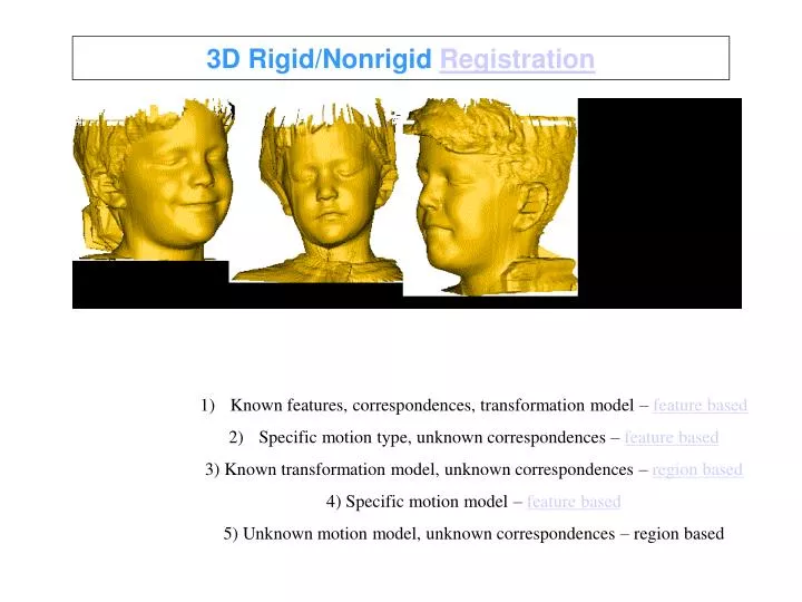
3D Rigid/Nonrigid Registration. Known features, correspondences, transformation model – feature based Specific motion type, unknown correspondences – feature based 3) Known transformation model, unknown correspondences – region based 4) Specific motion model – feature based

E N D
3D Rigid/Nonrigid Registration • Known features, correspondences, transformation model – feature based • Specific motion type, unknown correspondences – feature based • 3) Known transformation model, unknown correspondences – region based • 4) Specific motion model – feature based • 5) Unknown motion model, unknown correspondences – region based
Visual Motion Jim Rehg (G.Tech)
Motion (Displacement) of Environment Image plane Scene Flow Motion Field Visual motion results from the displacement of the scene with respect to a fixed camera (or vice-versa). Motion field is the 2-D velocity field that results from a projection of the 3-D scene velocities
Applications of Motion Analysis • Visual tracking • Structure recovery • Robot (vehicle) navigation
Applications of Motion Analysis • Visual tracking • Structure recovery • Robot (vehicle) navigation
Motion Segmentation • Where are the independently moving objects (and how many are there)?
Optical Flow • 2-D velocity field describing the apparent motion in an image sequence • A vector at each pixel indicates its motion (between a pair of frames). Horn and Schunk Ground truth
Optical Flow and Motion Field • In general the optical flow is an approximation to the motion field. • When the scene can be segmented into rigidly moving objects (for example) the relationship between the two can be made precise. • We can always think of the optical flow as summarizing the temporal change in an image sequence.
Computing Optical Flow Courtesy of Michael Black
Cost Function for Optical Flow Courtesy of Michael Black
Lucas-Kanade Method • Brute-force minimization of SSD error can be inefficient and inaccurate • Many redundant window evaluations • Answer is limited to discrete u, v pairs
Lucas-Kanade Method • Problems with brute-force minimization of SSD error • Many redundant window evaluations • Answer is limited to discrete u, v pairs • Related to Horn-Schunk optical flow equations • Several key innovations • Early, successful use of patch-based model in low-level vision. Today these models are used everywhere. • Formulation of vision problem as non-linear least squares optimization, a trend which continues to this day.
Quality of Image Patch • Eigenvalues of the matrix contain information about local image structure • Both eigenvalues (close to) zero: Uniform area • One eigenvalue (close to) zero: Edge • No eigenvalues (close to) zero: Corner
Contributions of Lucas-Kanade • Basic idea of patch or template is very old (goes back at least to Widrow) • But in practice patch models have worked much better than the alternatives: • Point-wise differential equations with smoothness • Edge-based descriptions • Patchs provide a simple compact enforcement of spatial continuity and support (robust) least-squares estimators.
Summer School 2005 Medical Image Registration (a short overview) Alain Pitiot, Ph.D. Siemens Molecular Imaging - Advanced Applications
SOME APPLICATIONS • Medical Image Registration
Motivation • Advances in imaging technology novel modalities • see beyond: inside (non-invasive), • during (dynamic processes), • at small scale (increased resolution) • Understanding and correlating structure & function • - automated/aided diagnosis • - image guided surgery/radio-therapy • - treatment/surgery planning • - medical atlases • - longitudinal studies: disease progression, development
Definitions • Def. #1:put two images into spatial correspondence • goal: extract more/better information • Def. #2: maximize similarity between transformed source image & target image source image target image + transformed target image CT (thorax) PET (thorax) Anatomical Functional
Taxonomy • Nature of application • Subject • - intrasubject • - intersubject • - atlas Homer Simpson (MRI, coronal section)
Taxonomy • Nature of application • Subject • - intrasubject • - intersubject • - atlas Homer Simpson (monkey position) Homer Simpson (rest position) very similar shapes
Taxonomy • Nature of application • Subject • - intrasubject • - intersubject • - atlas Homo sapiens sapiens brain Homer Simpson expect larger differences
Taxonomy • Nature of application • Subject • - intrasubject • - intersubject • - atlas Homer Simpson (MRI) Homer Simpson (labelled atlas)
Taxonomy • Nature of application • Subject • - intrasubject • - intersubject • - atlas • Registration basis • - extrinsic • - intrinsic
Taxonomy • Nature of application • Subject • - intrasubject • - intersubject • - atlas • Registration basis • - extrinsic • - intrinsic fast, explicit computation prospective, often invasive, often rigid transf. only stereotactic frame
Taxonomy • Nature of application • Subject • - intrasubject • - intersubject • - atlas • Registration basis • - extrinsic • - intrinsic versatile, minimally invasive no ground truth PET scintillography
Taxonomy | Nature of Application • Registration basis extrinsic intrinsic • - landmark based • - segmentation based • - voxel based CT PET fast accuracy limited by localization precision
Taxonomy | Nature of Application • Registration basis extrinsic intrinsic • - landmark based • - segmentation based • - voxel based segmented corpora callosa fast accuracy limited by segmentation combine with voxel based
Taxonomy | Nature of Application • Registration basis extrinsic intrinsic • - landmark based • - segmentation based • - voxel based cryo. section myelin-stained histological section most flexible approach resource intensive combine with previous techniques
Taxonomy • Nature of input images • Modality • Combination: • - mono-modal: same modality for source and target • - multi-modal: different modality • Dimensionality • - spatial: 2-D/2-D, 2-D/3-D, 3-D/3-D • - temporal a few imaging modalities
Taxonomy global local • Constraints • fusion maximize similarity between • transformed source & target • Transformation space • - flexibility • rigid, affine, parameterized, • free-form • - support • local, global rigid affine parameterized fluid/elastic choose space that fits anatomy and/or application
Taxonomy • Constraints • Similarity measure • “intensities of matched images • verify criterion” • - to each hypothesis its measure: conservation affine functional statistical • conservation of intensity SSD • affine relationship correlation coefficient • functional relationship correlation ratio • statistical dependence mutual information source target
Taxonomy • Constraints • Similarity measure • “intensities of matched images • verify criterion” • - to each hypothesis its measure: conservation affine functional statistical • conservation of intensity SSD • affine relationship correlation coefficient • functional relationship correlation ratio • statistical dependence mutual information source target
Taxonomy • Constraints • Similarity measure • “intensities of matched images • verify criterion” • - to each hypothesis its measure: conservation affine functional statistical • conservation of intensity SSD • affine relationship correlation coefficient • functional relationship correlation ratio • statistical dependence mutual information source target
Taxonomy • Constraints • Similarity measure • “intensities of matched images • verify criterion” • - to each hypothesis its measure: conservation affine functional statistical • conservation of intensity SSD • affine relationship correlation coefficient • functional relationship correlation ratio • statistical dependence mutual information source target
Taxonomy • Constraints • Similarity measure • “intensities of matched images • verify criterion” • - to each hypothesis its measure: conservation affine functional statistical • conservation of intensity SSD • affine relationship correlation coefficient • functional relationship correlation ratio • statistical dependence mutual information source target
Taxonomy • Optimization • Often iterative • - deterministic • gradient descent • - stochastic • simulated annealing
Taxonomy • Optimization • Often iterative • - deterministic • gradient descent • - stochastic • simulated annealing
Taxonomy • Optimization • Often iterative • - deterministic • gradient descent • - stochastic • simulated annealing
Taxonomy • Optimization • Often iterative • - deterministic • gradient descent • - stochastic • simulated annealing • Heteroclite bag of tricks • - progressive refinement • - multi-scale (multi-resolution)
Taxonomy • Optimization • Often iterative • - deterministic • gradient descent • - stochastic • simulated annealing • bag of tricks • - progressive refinement • - multi-scale (multi-resolution)