Download
1 / 17
170 likes | 369 Views
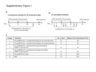
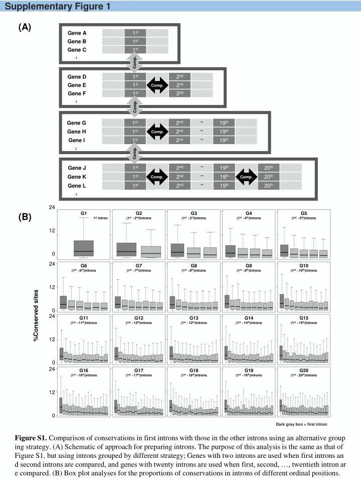
Supplementary Figure 1. (A). Comp. Comp. Comp. Comp. Comp. Comp. Comp. (B). Dark gray box = first intron.

E N D
Supplementary Figure 1 (A) Comp. Comp. Comp. Comp. Comp. Comp. Comp. (B) Dark gray box = first intron Figure S1. Comparison of conservations in first introns with those in the other introns using an alternative grouping strategy. (A) Schematic of approach for preparing introns. The purpose of this analysis is the same as that of Figure S1, but using introns grouped by different strategy; Genes with two introns are used when first introns and second introns are compared, and genes with twenty introns are used when first, second, …, twentieth intron are compared. (B) Box plot analyses for the proportions of conservations in introns of different ordinal positions.
Supplementary Figure 2 (A) H1-hesc (B) K562 DHS 40 TFBS 30 DHS 70 TFBS 30 20 15 35 15 0 0 0 0 100 100 100 100 H3K4me1 H3K4me3 H3K4me1 H3K4me3 50 50 50 50 % Signals % Signals 0 0 0 0 12 12 50 100 CTCF H3K9me3 CTCF H3K9me3 6 6 25 50 0 0 0 0 Introns grouped by their ordinal positions Introns grouped by their ordinal positions Figure S2. Proportions of regulatory chromatin marks in intron ordinal groups in H1-hESC and K562. Please refer to the legends of Figure S2. (A) Comparison of the proportions of the chromatin marks among different ordinal positions of introns in H1-hESC cell line, and (B) Comparison of the proportions of the chromatin marks among different ordinal positions of introns in K562 cell line.
Supplementary Figure 3 (A) H1-hesc (B) K562 Figure S3. Correlation between regulatory signals and conservation in first introns in H1-hESC and K562. Please refer to the legends of Figure 3. (A) Comparison between the proportions of the regulatory marks and the conservation in first introns in H1-hESC cell line, and (B) Comparison between the proportions of the regulatory marks and the conservation in first introns in K562 cell line.
Supplementary Figure 4 (A) GM12878 (B) H1-hesc (C) K562 Figure S4. Correlation between regulatory signals and conservation in the upstream flanking regions in three different cell lines. Please refer to the legends of Figure S3. Comparison of the proportions of conserved sites and regulatory signals for upstream in GM12878 cell line, (B) H1-hESC cell line, and (C) K562 cell line.
Supplementary Figure 5 Groups of genes containing each number of exon Figure S5. Relationship between flanking region conservation and the numbers of exons. Please refer to the legends of Figure S4. The proportions of conservation in upstream (left) and in downstream (right) of genes are compared with those with more than one exon, more than two exons, more than three exons, up to more than twenty exons.
Supplementary Figure 6 (A) From H1-hesc Groups of genes containing different numbers of exons Figure S6. Relationship between the proportions of regulatory signals in introns of each ordinal position and the numbers of exons. Please refer to the legends of Figure S5. Comparison between the proportions of active chromatin marks and the numbers of exons within genes in (A) H1-hESC cell line.
Supplementary Figure 6 (B) From K562 Groups of genes containing different numbers of exons Figure S6. Relationship between the proportions of regulatory signals in introns of each ordinal position and the numbers of exons. Please refer to the legends of Figure S5. Comparison between the proportions of active chromatin marks and the numbers of exons within genes in (B) K562 cell line.
Supplementary Figure 7 (A) UCSC_Refseq_mRNA (Jan 2013) 36,024 transcripts Transcripts with Intron Dataset of results 29,687 transcripts 1 gene – 1 transcript Gene2refseq (Nov 2013) ftp://ftp.ncbi.nlm.nih.gov/gene/DATA/ (B) Unique transcript harboring introns for a gene 16,374 transcripts (C) Groups of genes containing each number of exons Figure S7. Analysis based on a single representative transcript for each gene. (A) Schematic illustrating data preparation. Among the 36,024 transcripts downloaded from UCSC genome browser, a total of 29,687 transcripts are found to harbor at least one intron. Based on the transcript information using ‘Gene2Refseq’ obtained from ftp://ftp.ncbi.nlm.nih.gov/gene/DATA, for each gene with multiple transcripts, the longest transcript is retrieved, resulting in a total of 16,374 transcripts. (B)-(D) correspond to Figures S1,S4,S5 respectively, reanalyzed with the smaller set of transcripts. Please refer to the legends of those figures. Figure (D) is in next page.
Supplementary Figure 7 (D) Groups of genes containing different numbers of exons
Supplementary Figure 8 (A) From H1-hESC From K562 (B) Figure S8. Enrichment of regulatory marks in the first intron in two additional cell lines. Please refer to the legend for Figure S7. Log-odds ratio analysis is performed for enrichment of regulatory signals in conserved regions in the first intron in (A) H1-hESC cell line, (B) K562 cell line.
Supplementary Figure 9 (A) Histogram and Box-plot of first intron length Median ≤ 10183 transcripts (B) 5’ - Bins- 3’ Figure S9. Five prime to three prime biases in signal density along the first intron. (A) Schematic illustrating data preparation. Genes harboring short first introns (shorter than the median length) of each intron are excluded. (B) The proportions of various signal densities are estimated over entire first intron. The first intron is binned into five equal-sized bins. Then the fraction of each signal is estimated for each bin, and the fraction of introns in which the highest signal is a particular bin is shown.
Supplementary Figure 10 (A) 14 different ranking patterns in the sizes of the histone mark signals located in promoter, 1st exon, and 1st intron 5’FR 1st Exon 1st Intron The numbers of transcripts corresponding to each pattern for each signal Candidates for spill-overs 1 1 1 1 1 1 1 1 1 0 1 1 1 1 1 1 0 1 1 1 1 1 1 1 1 1 1 1 0 2 2 2 2 2 2 2 2 2 2 2 2 2 2 2 2 2 2 2 2 2 3 Stars for p-value < 0.001 one-sided Wilcoxon rank sum tests between the first intron and other downstream introns ( 2nd ~ 20th) 3 3 3 3 3 3 (B) (C) Groups of genes containing each number of exons
Supplementary Figure 10 (D) Groups of genes containing different numbers of exons Figure S10. Excluding spillover of signals s from the promoter. (A) The top panel illustrates spillover definition. Briefly, the sizes of the signal proportions are ranked among promoter, exon, and first intron in a transcript. For example, a transcript with the highest proportion of a signal in the promoter, the next lower proportion in the first exon, and the smallest proportion in the first intron is defined as a ‘P123’ set, and a transcript with the same levels of the proportions in all the three different structures is defined as a ‘P111 set’. A total of 14 different sets are defined by this ranking strategy, and five sets, i.e., P111, P112, P212, P122, and P123 are considered as spillovers. The bottom table shows the numbers of transcripts corresponding to each pattern where the sets colored red indicate spillovers. (B) Rebuilt Figure S1 after removing the introns with potential spillover, (C) Rebuilt Figure S4 after excluding potential spillover cases, and (D) Rebuilt Figure S5 after excluding potential spillover cases.
Supplementary Figure 11 (A) 3’ 5’ 5’FR 1st Exon 1st Intron 2nd Exon 2nd Intron 5’FR 5’FR 5’FR Exons Exons Exons 3’FR 3’FR 3’FR Antisense strand 5’ 3’ 5’FR Exons 3’FR 5’FR Exons 3’FR 5’FR Exons 3’FR Sense strand (B) (C) Groups of genes containing each number of exons
Supplementary Figure 11 (D) Groups of genes containing different numbers of exons Figure S11. Excluding genes whose first introns overlapped with exons or flanks of another genes. (A) Schematic showing the possible structural overlaps among different genes. (B) Rebuilt Figure S1B from “non-overlapped” datasets, (C) Rebuilt Figure 4 from “non-overlapped” dataset, and (D) Rebuilt Figure S5 from “non-overlapped” dataset.
Supplementary Figure 12 (A) TSS-distances from first introns 1st 1st Exon 1st Intron 2nd Exon 2nd Intron TSS TSS-distances from second introns 2nd Frequency 1st 2nd Distances (bp) Figure S12. Analyzing the effect of proximity to the TSS. (A) Histograms showing overlap in the distribution of distance from TSS for the first and the second introns. Please refer to the legends of Figure S8 for (B) and (C). (B) The same analysis as for Figure S8 from H1-hESC cell line, and (C) The same analysis as for Figure S8 from K562 cell line. Figures (B) and (C) are in next page.
Supplementary Figure 12 (B) From H1-hesc (A) (B) (C) FromK562 (A) (B)