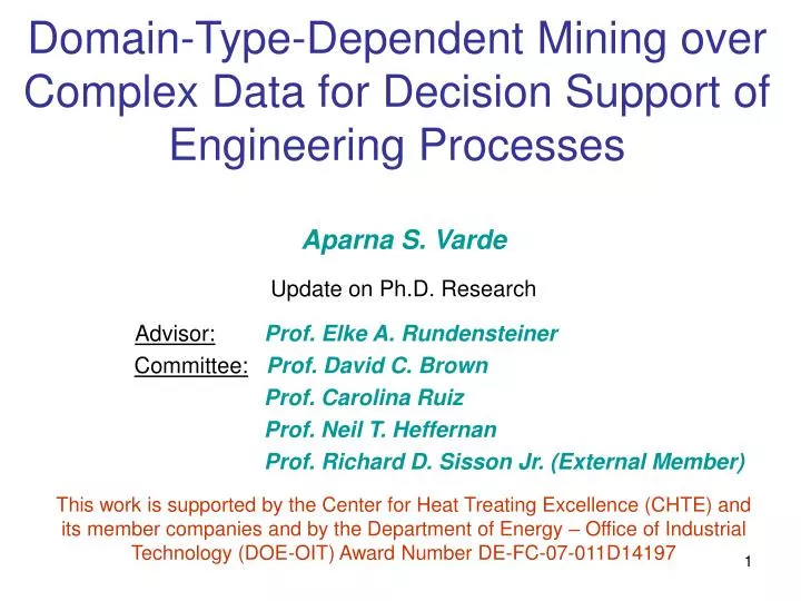
Domain-Type-Dependent Mining over Complex Data for Decision Support of Engineering Processes

1. Domain-Type-Dependent Mining overComplex Data for Decision Support of Engineering Processes Aparna S. Varde Update on Ph.D. Research Advisor:Prof. Elke A. Rundensteiner Committee:Prof. David C. Brown Prof. Carolina Ruiz Prof. Neil T. Heffernan Prof. Richard D. Sisson Jr. (External Member) This work is supported by the Center for Heat Treating Excellence (CHTE) and its member companies and by the Department of Energy – Office of Industrial Technology (DOE-OIT) Award Number DE-FC-07-011D14197

2. Motivation • Experimental data in a domain used to plot graphs. • Graphs: good visual representation of results of experiments. Expt. Expt • Performing experiment consumes time and resources. • Users want to estimate results, given input conditions. • This helps in decision support in the domain. • Also want to estimate input conditions, given results. • This motivates development of a technique for this estimation. • Assumption: Previous data (input + results) stored in database.

3. Proposed Approach: AutoDomainMine • Cluster experiments based on graphs (results). • Learn clustering criteria (combination of input conditions that characterize clusters). • Use criteria learnt as the basis for estimation.

4. AutoDomainMine: Clustering

5. AutoDomainMine: Estimation

6. Approach: Why Cluster Graphs • Why not cluster input conditions, and learn clustering criteria? • Problem: This gives lower accuracy than clustering graphs. • Reason: • Clustering technique attaches same weight to all conditions. • This adversely affects accuracy. • Cannot be corrected by introducing relative weights. • Since weights are not known in advance. • They depend on relative importance of conditions. • Relative importance of conditions learnt from results. • Hence, more feasible to cluster based on graphs (results).

7. Clustering Techniques • Various clustering techniques: K-means, EM, COBWEB etc. • K-means preferred for AutoDomainMine • Partitioning-based algorithm. • K-means is simplistic and efficient. • It gives relatively higher accuracy. • Process of K-Means [Witten et. al.] • Repeat • K points chosen as random cluster centers. • Instances assigned to closest cluster center by “distance”. • Mean of each cluster calculated. • Means form new cluster centers. • Until same points assigned to each cluster in consecutive iterations. • Notion of “distance” crucial. K-means Clustering

8. Types of Distance Metrics • In original space of objects, categories of distance metrics in the literature [Keim et. al]. • Position-based • Actual location of objects, e.g, Euclidean Distance. • Statistical • Significant observations, e.g. Mean distance. • Others • Appearance and relative placement of objects, e.g. Tri-plots [Faloustos et.al.]

9. Position-based distance: Examples The ‘city-block’ distance. Manhattan distance bet. point P (P1, P2 … Pn) and point Q (Q1, Q2 … Qn) is: The ‘as-the-crow-flies’ distance. Euclidean distance bet. point P (P1, P2 … Pn) and point Q (Q1, Q2 … Qn) is: D = Σ i =1 to n |Pi – Qi| D = √Σ i =1 to n (Pi – Qi)^2

10. Statistical Distance: Examples • Types based on statistical observations. [Petrucelli et. al] • Mean distance between graphs A and B • Dmean(A,B) = |μ(A) – μ(B)| • Maximum distance • Dmax(A,B) = |Max(A) – Max(B)| • Minimum distance • Dmin(A,B) = |Min(A) – Min(B)| • Define distance-type based on “Critical Points”, e.g., Leidenfrost Pt. • Dcp(A,B) = |Critical_Point(A) – Critical_Point(B)|, e.g., DLF (A, B) shown. DLF(A,B) Graph A Graph B

11. Clustering Graphs • DefaultDistance Metric: Euclidean Distance. • Problem:Graphs below placed in same cluster, relative to other • curves. Should be in different clusters as per domain. • Learn domain specific distance metric for accurate clustering.

12. General Definition of Distance Metric in AutoDomainMine • Distance metric defined in terms of • Weights*Components • Components: Position, Statistical aspects, Others. • Subtypes of each • Weights: Numerical values • Relative importance of each component • Formula: Distance “D” defined as, • D = w1*c1 + w2*c2 + …….. wn*cn • D = Σ{s=1 to n} ws*cs • Example • D = 4*Euclidean + 3*Mean + 5*Critical_Point

13. Learning the Metric • Training set: Correct clusters of graphs. • As verified by domain experts • Basic Process: • Guess initial metric • Do clustering • Evaluate accuracy • Adjust and re-execute / Halt • Output final metric • Alternatives: A. With Additional Domain Expert Input B. No Additional Input

14. Alternative A: Guess Initial Metric • Domain Expert Input: Select components based on significant aspects in domain. • Position, Statistical, Others. • Subtypes in each category. • One or more aspects / subtypes selected. • Example of User Input • Euclidean, Mean, Critical Points. • Consider this as guess of components. • Randomly guess initial weights for each component. • Thus define initial metric. • Example • D = 4*Euclidean + 3*Mean + 5*Critical_Point

15. Alternative A: Do Clustering • Use guessed metric as “distance” in clustering. • Perform clustering using k-means. • Repeat • K points chosen as random cluster centers. • Instances assigned to closest cluster center by “D = Σ{s=1 to n} w*c” • Mean of each cluster calculated. • Means form new cluster centers. • Until same points assigned to each cluster in consecutive iterations.

16. Alternative A: Evaluate Accuracy • Measure Error(E) between predicted & actual clusters. • E α D(p,a) with this metric • where p: predicted & a:actual cluster. • Error Functions: If “n” is number of clusters, • Mean squared error • E = [ (p1-a1)^2 + …. + (pn-an)^2 ] / n • Root mean squared error • E = √ { [ (p1-a1)^2 + …. + (pn-an)^2 ] / n } • Mean absolute error • E = [ |p1-a1| + …. + |pn-an| ] / n • AutoDomainMine selects error function based on type of position-distance (Euclidean / Manhattan etc.)

17. Alternative A: Adjust & Re-execute / Halt • Use error to adjust weights of components for next iteration. • Apply general principle of error back-propagation. • Thus make next guess for metric. • Example • Old D = 4*Euclidean + 3*Mean + 5*Critical_Point • New D = 5*Euclidean + 1*Mean + 6*Critical_Point • Use this guessed metric to re-do clustering. • Repeat Until error is minimum OR max # of epochs reached. • Ideally error should be zero.

18. Alternative A: Output Final Metric • If error minimum, then distance D gives high accuracy in clustering. • Hence output this D as learnt distance metric. • Example • D = 3*Euclidean + 2*Mean + 6*Critical_Point

19. Alternative B • No domain expert input about significant aspects. • Use principle of Occam’s Razor to guess metric.[Russell et. al.] • Select simplest hypothesis that fits the data. • Example: Initially guess only Euclidean distance. • D = 1*Euclidean • Do clustering and evaluate accuracy as in Alternative A. • To adjust and re-execute • Pass 1: Alter weights. Repeat as in alternative A until error min. OR max. # of epochs. • Pass 2: Add one component at a time. Repeat whole process until error min. OR max. # of epochs. • Output corresponding metric D as learnt distance metric.

20. Comments on Learning the Metric • Clustering with test sets will be done to evaluate the learnt metric. • Learning method subject to change • based on results of clustering with test sets. • Possibility: Some combination of alternatives A & B. • Other learning approaches being considered.

21. Dimensionality Reduction • Each graph has thousands of points. Dimensionality reduction needed. • Random Sampling [Bingham et. al.] • Consider points at regular intervals, e.g., every 10th point, • Include all significant points, e.g., peaks. Random Sampling • Fourier Transforms [Blough et. al.] • Map data from time to frequency domain. • Xf = (1/√n)Σ{t = 0 to n-1} exp(-j2πft/n) where f = 0,1… (n-1) and j = √ -1 • Retaining first 3 to 5 Fourier Coefficients enough. • Fourier Transforms more accurate • In heat treating domain, proved experimentally. • In other domains, Fourier Transforms popular for storing / indexing data. [Wang et. al.] Fourier Transforms

22. Some inaccuracy still persists Should be in Cluster A Cluster A Cluster B

23. Map Learnt Metric to Reduced Space • Distance metric learnt in original space. • Map learnt metric to reduced vector space. • Derive formulae using Fourier Transform properties. • Example: Euclidean Distance (E.D.) is preserved during Fourier Transforms. [Agrawal et. al.] • E.D. in time domain • D(x,y) = 1/n [ √ (Σ{t = 0 to n-1} |x_t – y_t|^2) ] • E.D. in frequency domain • D(X,Y) = 1/n [ √ (Σ{f = 0 to n-1} |X_f – Y_f|^2) ]

24. Properties useful for mapping • Some properties of Fourier Transforms useful for mapping. [Agrawal et. al.] • Energy Preservation • Parseval’s Theorem: Energy in time domain ~ energy in frequency domain. • Thus, ∑ {t= 0 to n-1} (| xt | ^2) = ∑{f= 0 to n-1} (| Xf | ^2) • Linear Transformation • “t” is time domain, “f” is frequency domain • [xt]  [Xf] means that Xf is a Discrete Fourier Transform of xt. • Discrete Fourier Transform is a Linear Transformation. Thus, • If [xt]  [Xf]; [yt]  [Yf] • then [xt + yt]  [Xf + Yf] • and [axt]  [aXf] • Amplitude Preservation • Shift in time domain changes phase of Fourier coefficients, not amplitude. • Thus, [x(t-t0)]  [ Xf exp (2πft0 / n) ] • Euclidean Distance (E.D.) Preservation • E.D. between signals, x` and y` in time domain ~ E.D. in frequency domain. • Thus, || xt` – yt` || ^ 2 ~ || Xf` - Yf`|| ^ 2

25. Clustering with Learnt Metric Example of desired clusters: as expected to be produced with learnt distance metric

26. Issues to be addressed • Learning clustering criteria. • Designing representative cases. • Re-Clustering for maintenance to enhance estimation accuracy.

27. Learning Clustering Criteria • Classification used to learn the clustering criteria • combinations of input conditions that characterize clusters. • Decision Tree Induction: classification method [Russell et. al.] • Good representation for categorical decision making. • Eager learning. • Provides reasons for decisions. • With existing clusters ID3 [Quinlan et. al.] gives lower accuracy. • J4.8 [Quinlan et. al.] gives higher accuracy with same clusters. • Better clusters with domain specific distance metric likely to enhance classifier accuracy. Sample Partial Decision Tree

28. Designing Representative Cases • Clustering criteria used to form representative case • One set of input conditions and graph for each cluster • Selecting arbitrary case not good • May not incorporate significant aspects of cluster. • E.g, several combinations of input conditions may lead to one graph. • Average of conditions not good • E.g., consider condition A1 = “high” and B1 = “low”, • Common condition AB1 = “medium” is not a good representation. • Average of graphs not good • Some features on the graph may be more significant than others. • Challenge: Design “good” representative case as per domain.

29. Re-Clustering for Maintenance • New data gets added to system. Its effect should be incorporated. • Clustering should be done periodically, as more tuples are added to the database, representing new experiments. • This is to enhance the accuracy of the learning. New set of clusters, new clustering criteria for better estimation. • Should new distance metric be learnt with additional data? • VLDB issues: Database layout, multiple sources, multiple relations per source, clustering in this environment.

30. Contributions of AutoDomainMine • Learning a domain specific distance metric for accurate clustering and mapping the metric to a new vector space after dimensionality reduction. • Designing a good representative case per cluster after accurately learning the clustering criteria. • Re-Clustering for maintenance as more data gets added to enhance estimation accuracy.

31. Related Work • Naïve similarity searching / exemplar reasoning. [Mitchell et. al.] • Instance Based Reasoning with feature vectors. [Aamodt et. al.] • Case Based Reasoning with the R4 cycle. [Aamodt et. al.] • Integrating Rule Based & Case Based approaches. [Pal et. al.] • Mathematical modeling in the domain. [Mills et. al.]

32. Naïve Similarity Searching • Based on exemplar reasoning. [Mitchell et. al.] • Compare input conditions with existing experiments. • Select closest match (number of matching conditions). • Output corresponding graph. • Problem: Condition(s) not matching may be most crucial. • Possible Solution: Weighted similarity search, i.e., Instance Based Reasoning with Feature Vectors…

33. Instance Based Reasoning: Feature Vectors • Search guided by domain knowledge. [Aamodt et. al.] • Relative importance of search criteria (input conditions) coded as weights into feature vectors. • Closest match is number of conditions along with weights. • Problem: Relative importance of criteria not known w.r.t. impact on graph. • E.g., excessive agitation more significant than a thin oxide layer, • Moderate agitation may less significant than a thick oxide layer. • Need to learn relative importance of criteria from results of experiments.

34. Case Based Reasoning: R4 cycle • Case Based Reasoning (CBR) with R4 cycle [Aamodt et. al.] • Retrieve case from case base to match new case. • Reuse solution of retrieved case as applicable to new case. • Revise, i.e., make modifications to new case for a good solution. • Retain modified case in case base for further use. • When user submits new conditions to estimate graph • Retrieve input conditions from database to match new ones. • Reuse corresponding graph as possible estimation. • Revise as needed to output this as actual estimation. • Retain modified case (conditions + graph) in database for future use. • Problems • Requires excessive domain expert intervention for accuracy. • Is not a completely automated approach. • Is dependent on availability of domain experts. • Consumes too much time & resources.

35. Rule Based + Case Based Approach • General domain knowledge coded as rules. • Case specific knowledge stored in case base. • Two approaches combined could provide more accurate estimation in some domains, e.g., Law. [Pal et. al.] • Problems • Our focus: experimental data and graphical results. • Rules may help in estimating tendencies from graphs. • Not feasible to apply rules to estimate actual nature of graphs. • Several factors involved, hard to pinpoint which ones cause a particular feature on graph. • Hence not advisable to apply rule based reasoning.

36. Mathematical Modeling in Domain • Construct a model correlating input conditions to results. [Mills et. al.] • Representation of graphs in terms of numerical equations. • Needs precise knowledge of how inputs conditions affect graphical results. • Not known in many domains, hence not accurate estimation. • Example: • In heat treating, this modeling does not work for multiphase heat transfer with nucleate boiling. • Hence does not accurately estimate graph, especially in liquid quenching.

37. AutoDomainMine: Theoretical knowledge plus practical results • Combine both aspects • Fundamental domain knowledge • Results of experiments • Derive more advanced knowledge • Basis for estimation • Learning approach used in many domains • Automate this approach

38. Demo of Pilot Tool • http://mpis.wpi.edu:9006/database/autodomainmine/admintro1.html