Download
1 / 27
270 likes | 447 Views
6.853: Topics in Algorithmic Game Theory. Lecture 15. Fall 2011. Constantinos Daskalakis. Recap. Exchange Market Model. traders. divisible goods. trader i has:. - utility function. non-negative reals. consumption set for trader i.

E N D
6.853: Topics in Algorithmic Game Theory Lecture 15 Fall 2011 Constantinos Daskalakis
Exchange Market Model traders divisible goods trader i has: - utilityfunction non-negative reals consumption set for trader i specifies trader i’s utility for bundles of goods - endowment of goods amount of goods trader comes to the marketplace with
Fisher Market Model ntraders with: money mi ,and utility functionui kdivisible goods owned by seller; seller has qj units of good j can be obtained as a special case of an exchange market, when endowment vectors are parallel: in this case, relative incomes of the traders are independent of the prices.
Competitive (or Walrasian) Market Equilibrium Def: A price vector is called a competitive market equilibriumiff there exists a collection of optimal bundles of goods, for all traders i= 1,…, n, such that the total supply meets the total demand, i.e. total supply total demand [ For Fisher Markets: ]
Arrow-Debreu Theorem 1954 Theorem [Arrow-Debreu 1954]: Suppose (i) is closed and convex (ii) (all coordinates positive) (iii a) (iii b) (iii c) Then a competitive market equilibrium exists.
Fisher’s Model Suppose all endowment vectors are parallel… relative incomes of the traders are independent of the prices. Equivalently, we can imagine the following situation: n traders, with specified money mi k divisible goods owned by seller; seller has qj units of good j Arrow-Debreu Thm (under the Arrow-Debreu conditions) there exist prices that the seller can assign on the goods so that the traders spend all their money to buy optimal bundles and supply meets demand
Utility Functions CES (Constant Elasticity of Substitution) utility functions: linear utility form Leontief utility form Cobb-Douglas form
Fisher’s Model with CES utility functions • Buyers’ optimization program (under price vector p): • Global Constraint:
Eisenberg-Gale’s Convex Program • The space of feasible allocations is: • But how do we aggregate the trader’s optimization problems into one global optimization problem? e.g., choosing as a global objective function the sum of the traders’ utility functions won’t work…
Eisenberg-Gale’s Convex Program Observation: The global optimization problem should not favor (or punish) Buyer i should he • Double all her uij’ s • Split himself into two buyers with half the money • Eisenberg and Gale’s idea: Use the following objective function (take its logarithm to convert into a concave function)
Eisenberg-Gale’s Convex Program Remarks: - No budget constraints! - It is not necessary that the utility functions are CES; everything works as long as they are concave, and homogeneous
Eisenberg-Gale’s Convex Program KKT Conditions - interpret Langrange multipliers as prices - primal variables + Langrange multipliers comprise a competitive eq. 1. Gives a poly-time algorithm for computing a market equilibrium in Fisher’s model. 2. At the same time provides a proof that a market equilibrium exists in this model. Homework: Show 1, 2 for linear utility functions.
Back to the Exchange Model Complexity of market equilibria in CES exchange economies. -1 0 1 At least as hard as solving Nash Equilibria[CVSY ’05] Poly-time algorithms known [Devanur, Papadimitriou, Saberi, Vazirani ’02], [Jain ’03], [CMK ’03], [GKV ’04],… OPEN!!
Hardness of Leontief Exchange Markets Theorem [Codenotti, Saberi, Varadarajan, Ye ’05]: Finding a market equilibrium in a Leontief exchange economy is at least as hard as finding a Nash equilibrium in a two-player game. Corollary: Leontief exchange economies are PPAD-hard. Proof Idea: Reduce a 2-player game to a Leontief exchange economy, such that given a market equilibrium of the exchange economy one can obtain a Nash equilibrium of the two-player game.
Excess Demand at prices p suppose there is a unique demand at a given price vector p and its is continuous (see last lecture) We already argued that under the Arrow-Debreu Thm conditions: (H) f is homogeneous, i.e. (WL) f satisfies Walras’s Law, i.e. (we argued that the last property is true using nonsatiation + quasi-concavity, see next slie)
Justification of (WL) under Arrow-Debreu Thm conditions Nonsatiation + quasi-concavity local non-satiation at equilibrium every trader spends all her budget, i.e. if xi(p) is an optimal solution to Programi(p) then i.e. every good with positive price is fully consumed
Excess Demand at prices p suppose there is a unique demand at a given price vector p and its is continuous (see last lecture) We already argued that under the Arrow-Debreu Thm conditions: (H) f is homogeneous, i.e. (WL) f satisfies Walras’s Law, i.e.
Gross-Substitutability (GS) Def: The excess demand function satisfies Gross Substitutability iff for all pairs of price vectors p and p’: In other words, if the prices of some goods are increased while the prices of some other goods are held fixed, this can only cause an increase in the demand of the goods whose price stayed fixed.
Differential Form of Gross-Substitutability (GSD) Def: The excess demand function satisfies the Differential Form of Gross Substitutability iff for all r, s the partial derivatives exist and are continuous, and for all p: Clearly: (GSD) (GS)
Not all goods are free (Pos) Def: The excess demand function satisfies (Pos) if not all goods are free at equilibrium. I.e. there exists at least one good in which at least one trader is interested.
Properties of Equilibrium Lemma 1 [Arrow-Block-Hurwicz 1959]: Suppose that the excess demand function of an exchange economy satisfies (H), (GSD) and (Pos). Then if is an equilibrium price vector Suppose that the excess demand function of an exchange economy satisfies (H), (GS) and (E+). Then if and are equilibrium price vectors, there exists such that Call this property (E+) Lemma 2 [Arrow-Block-Hurwicz 1959]: i.e. we have uniqueness of the equilibrium ray
Weak Axiom of Revealed Preferences (WARP) Theorem [Arrow-Hurwicz 1960’s]: Suppose that the excess demand function of an exchange economy satisfies (H), (WL), and (GS). If >0 is any equilibrium price vector and >0 is any non-equilibrium vector we have Proof on the board
Computation of Equilibria Corollary 1 (of WARP): If the excess demand function satisfies (H), (WL), and (GS), it can be computed efficiently and is Lipschitz, then a positive equilibrium price vector (if it exists) can be computed efficiently. proof sketch: W. l. o. g. we can restrict our search space to price vectors in [0,1]k, since any equilibrium can be rescaled to lie in this set (by homogeneity of the excess demand function). We can then run ellipsoid, using the separation oracle provided by the weak axiom of revealed preferences. In particular, for any non-equilibrium price vector p, we know that the price equilibrium lies in the half-space