Download
1 / 55
550 likes | 714 Views
Group 1. Group 2. Airline ticket purchase. Airline ticket purchase. (time cost $0.50). (time cost $0.50). Reliability (re. -. test). Rotate. Rotate. 50% in . 50% in . Foraging costs . Generalizability. each . each . manipulation. group to . group to . cancel . cancel .

E N D
Group 1 Group 2 Airline ticket purchase Airline ticket purchase (time cost $0.50) (time cost $0.50) Reliability (re - test) Rotate Rotate 50% in 50% in Foraging costs Generalizability each each manipulation group to group to cancel cancel learning learning effect. effect. Car rental purchase Airline ticket purchase (time cost $0.50) (time cost $1.00) $0.75
Group 1 Group 2 Reliability Airline ticket purchase (NY – WAS) Airline ticket purchase (NY – WAS) Rotate Rotate 50% in 50% in Reliability Generalizability each each group to group to cancel cancel learning learning effect. effect. Car rental purchase (WAS) Airline ticket purchase (NY – SFO)
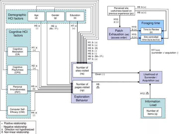
Table 6.3.1. Cognitive Absorption Correlation Matrix H1a: The CA score is positively related to the number of sites visited while foraging. Individuals with a high CA score are likely to visit more websites than those with low CA scores. H1b: The CA score is positively related to the number of pages accessed while foraging. Individuals with a high CA score are likely to visit more web pages within a site than those with low CA scores. • H1a: IS REJECTED • H1b: IS REJECTED
Table 6.3.2. Computer Playfulness Correlation Matrix H2a: The CPS score is positively related to the number of sites visited while foraging. Individuals with a high CPS score are likely to visit more web sites than those with low CPS scores. H2b: The CPS score is positively related to the number of pages accessed while foraging. Individuals with a high CPS score are likely to visit more web pages than those with low CPS scores. • H2a: IS REJECTED • H2b: IS REJECTED
Table 6.3.3. Personal Innovativeness with Information Technology Correlation Matrix H3a: Individuals with lower PIIT score is likely visit a different number of websites site than those with higher PIIT scores (no direction is hypothesized) H3b: Individuals with lower PIIT score is likely visit a different number of web pages within a site than those with higher PIIT scores (no direction is hypothesized) • H3a: IS SUPPORTED • H3b: IS SUPPORTED
Table 6.3.4. Computer Self-Efficacy Correlation Matrix H4a: The CSE score is negatively related to the number of sites visited while foraging. Individuals with a high CSE score are likely to visit fewer websites than those with low CSE scores. H4b: The CSE score is negatively related to the number of pages accessed while foraging. Individuals with a high CSE score are likely to visit fewer web pages than those with low CSE scores. • H4a: IS REJECTED • H4b: IS REJECTED
Table 6.3.5. Age Correlation Matrix H5a: Age is negatively related to the number of sites visited. Older individuals visit fewer websites than younger individuals. H5b: Age is negatively related to the number of pages visited. Older individuals visit fewer web pages than younger individuals. • H5a: IS REJECTED • H5b: IS REJECTED
Table 6.3.6b. T-scores Gender Difference of Means (assuming unequal variance) *97% confidence H6a: When foraging, males visit more websites than females. H6b: When foraging, males visit more web pages than females. • H6a: IS REJECTED • H6b: IS REJECTED, BUT SUPPORTED IN THE OPPOSITE DIRECTION (When purchasing on-line, males visit less web pages than females)
Table 6.3.7a. Education level and Observed Number of Websites visited. Table 6.3.7b. Education level and Expected Number of Websites visited. Based on this data we calculated a Chi-Squared value of 9.562 and 6 degrees of freedom [(k-1)*(n-1)]. Based on this, there appears to only an 85.5% confidence that differences in the number of websites visited exists between the various education levels H7a: Education level is positively related with the number of sites visited. Individuals with higher levels of education are more likely to visit more websites than those with lower levels of education. • H7a: IS REJECTED
Table 6.3.7c. Education level and Observed Number of Web pages visited. Table 6.3.7d. Education level and Expected Number of Web pages visited. Based on this data we calculated a Chi-Squared value of 14.861 and 6 degrees of freedom [(k-1)*(n-1)]. Based on this, we found that differences do in fact exists between the various education levels and the number of web pages accessed when buying on-line (99% confidence). H7b: Education level is positively related with the number of pages visited. Individuals with higher levels of education are more likely to visit more web pages than those with lower levels of education. • H7b: IS REJECTED, BUT SUPPORTED IN THE OPPOSITE DIRECTION (When purchasing on-line, higher educated individuals visit less web pages than those less educated)
Table 6.3.8a Non-Linear Prediction Model Accuracy of Purchases based on Web Pages visited H8: A non-linear relationship exists between the number of pages accessed and the likelihood of surrender. • H8: IS SUPPORTED
Figure 6.3.8b Predictive Probability distribution Based on web pages Visited
Table 6.3.9 Perceived Usefulness and Patch Exhaustion Correlation Matrix H9a: The perceived usefulness based on previous experience is positively related to the time a user will spend on reviewing search results at an e-commerce site. H9b: The perceived usefulness based on previous experience is positively related to the site time the user will spend at an e-commerce site (patch). (site time is defined as the foraging time less the reviewing time). • H9a: IS SUPPORTED • H9b: IS SUPPORTED
Table 6.3.10a Patch Exhaustion Correlation Matrix It is interesting to see that there are no significant correlations between the participant’s experience with a website and the order they access the sites. However, there is a significant correlation between the Perceived Usefulness rank of the websites and how the participants accessed the sites (r = 0.502, 99.9% confidence). This supports the Optimal Foraging Theory predictions from biology (Smith and Dawkins, 1971; Smith and Sweatman, 1974), which suggested that such as behavior should also be exhibited by humans. H10a: The order of access of a site is positively related with perceived usefulness based on previous experience. Users perform patch exhaustion based on perceived usefulness of sites based on previous experience. • H10a: IS SUPPORTED
Table 6.3.10b Access Order and Site time Correlation Matrix H10b: The order of site access is positively related to the time a person will spend reviewing search results. Users are accessing sites that they are willing to spend more time reviewing items from first. H10c: The order of site access is positively related to the site time the user will spend at an e-commerce site. Users are accessing sites that they are willing to spend more time at first (site time is defined as the foraging time less the reviewing time). Participants actually spent less time at the websites they accessed first, and more time at later sites. Since, we separated the ‘acquisition time’ in the analysis, the correlations does not originate by the fact that most purchases were done by the later websites. The reason for this finding may be due to the ‘state of mind’ by the participants when executing a search. Initially, a person may be in an exploration mode where the focus is on exploration breath and the belief that more websites should be examined. As a result, less time may be devoted to the first websites visited. At subsequent websites, this desire may have been met and the individual become more focused on exploration depth. • H10b: IS REJECTED BUT SUPPORTED IN THE OPPOSITE DIRECTION (user spent less time reviewing items offered for sale at websites they access first, more at subsequent sites) • H10c: IS REJECTED BUT SUPPORTED IN THE OPPOSITE DIRECTION (user spent less time at websites they access first and more at subsequent sites)
H11a: The time to access a web page is positively related with the likelihood of site surrender and negatively related with the likelihood of acquisition. The longer a web page takes to load, the more likely that it will be abandoned and the less likely that the user will make a purchase from it. H11b: The time needed to orient at a web page is positively related with the likelihood of site surrender and negatively related with the likelihood of acquisition. The longer it takes to orient, the more likely that it will be abandoned and the less likely that the user will make a purchase from it. H11c: The time needed to enter a search at a web page is positively related with the likelihood of site surrender and negatively related with the likelihood of acquisition. The longer it takes to enter all required search criteria, the more likely that it will be abandoned and the less likely that the user will make a purchase from it. H11d: The time needed to execute a search at a web page is positively related with the likelihood of site surrenders and negatively related with the likelihood of acquisition. The longer it takes to execute a search, the more likely that it will be abandoned and the less likely that the user will make a purchase from it. H11e: The time needed to review the results from a website is positively related with the likelihood of site surrender and negatively related with the likelihood of acquisition. The longer it takes to review items from a search, the more likely that it will be abandoned and the less likely that the user will make a purchase from it.
Table 6.3.11a Binary Regression Coefficients for Predicted Buy Vs. Don’t Buy Decisions (first step) is P(x) = B0 + β1*X1 + β2*X2+…. βn*Xn . Where P(x) is defined as the probability that a binomial value is set (P(x)>0.5 = 1 and P(x)<0.5 = 0). • H11a: IS REJECTED
Table 6.3.11b Binary Regression Coefficients for Predicted Buy Vs. Don’t Buy Decisions (second and final step) Figure 6.3.11a Final Binary Regression Model for Predicted Buy Vs. Don’t Buy Decisions P(x) = -15.887 + 7.401 * time to orient - 0.269 * time to enter - 1.305 * time to find + 0.019 * time to review Table 6.3.11c Airline Ticket Purchasing Binary Logistic Regression Model Accuracy based on Time Factors
H11b: IS REJECTED BUT SUPPORTED IN THE OPPOSITE DIRECTION (the longer it takes to orient, the less likely that a website will be abandoned and the more likely that the user will make a purchase from it). • H11c: IS SUPPORTED • H11d: IS SUPPORTED • H11e: IS REJECTED BUT SUPPORTED IN THE OPPOSITE DIRECTION (the longer a person spend reviewing items at a site, the less likely that a website will be abandoned and the more likely that the user will make a purchase from it).
Figure 6.3.12a Generalized Predictive Purchasing Equations given: given: given: P(x) - the probability that a purchase will take place at a given site with x number of items x - the number of items available for purchasing on a website after a search β - the discriminate beta factor (context specific i.e. for car rentals, airline ticket purchasing) e - error rate of the model ε - the number of incorrectly predicted binomal values (buy/surrender) η - the number of correctly predicted binomal values (buy/surrender) ρ - the predictable power of the equation σ - the standard deviation of the probability q - the probability that a purchase will not occur at this type of site [1-P(x)] n - number of web pages visited H12: There is a non-linear relationship between the number of items returned by a search and the likelihood of surrender from a site
Figure 6.3.12b Predictive Purchasing Equation for Car rentals Figure 6.3.12c Discrete Betas of Car Rentals based on Number of Sales Items on a Web page
Figure 6.3.12d Predictive Purchasing Equation for Airline Ticket Purchases Figure 6.3.12c Discrete Betas of Airline Ticket sales based on Number of Sales Items on a Web page
Figure 6.3.12f Confidence Intervals of web pages accessed Prior to Purchase of based on Number of Airline Tickets on a Web page • H12: IS SUPPORTED
Figure 6.3.13a Cox and Snell’s R-Square Equation Figure 6.3.13b Nagelkerke R-Square Equation
Sample Data Model Type Model Validation For Model Build Predictive Linear Model Test of Model accuracy against sample (170 site visits) Site visit: sample of 170 from 1,134 site visits Explanatory Linear Model Test of Model accuracy against remaining observations (964 site visits) Predictive Non-Linear Model Test of Model accuracy against sample (51 site visits by unique visitors) Predictive Linear Model Individuals: sample of 51 from 151site visits by unique visitors (one sample per participant) Test of Model accuracy against remaining observations (100 site visits by unique visitors) Explanatory Linear Model
Overall differences - Flight #1 = $0.50 search cost per minute Flight #2 is $0.75 search costs per minute)
Overall differences - Flight #1 = $0.50 search cost per minute Flight #2 is $0.75 search costs per minute)
Overall differences - Flight #1 = $0.50 search cost per minute Flight #2 is $0.75 search costs per minute)
Overall differences - Flight #1 = $0.50 search cost per minute Flight #2 is $0.75 search costs per minute)