Materials Process Design and Control Laboratory

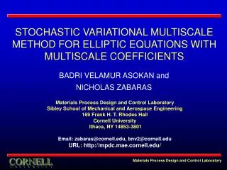
1. A STOCHASTIC VARIATIONAL MULTISCALE METHOD WITH EXPLICIT SUBGRID MODELING FOR ADVECTION-DIFFUSION SYSTEMS NICHOLAS ZABARAS and B. VELAMUR ASOKAN Materials Process Design and Control Laboratory Sibley School of Mechanical and Aerospace Engineering169 Frank H. T. Rhodes Hall Cornell University Ithaca, NY 14853-3801 Email: zabaras@cornell.edu, bnv2@cornell.edu URL: http://mpdc.mae.cornell.edu/

2. OUTLINE • Stochastic variational multiscale method • Uncertainty modeling – Overview and techniques • Stochastic advection-diffusion systems – ASGS modeling • Stochastic fluid-flow – ASGS modeling • Stochastic natural-convection – capturing unstable equilibrium • Stochastic multiscale elliptic equation • Stochastic multiscale advection-diffusion • Extensions and future research

3. MULTISCALE TRANSPORT SYSTEMS Fluid-flow Solidification Diffusion in composites • Presence of various spatial and temporal length scales • Varied application areas – Engineering, Material science and other • Uncertainty manifests from impreciseness in boundary condition, material property specification and other modeling assumptions

4. IMPORTANCE OF UNCERTAINTY • Propagation and interaction of uncertainties have to be resolved Meso Component Imprecise boundary conditions, initial perturbations Imprecise knowledge of governing model micro Only statistical description of material properties possible

5. MODELING ASPECTS OF UNCERTAINTY • Probabilistic interpretation – Imprecise knowledge about boundary conditions, governing models, material properties described using stochastic processes • Uncertainty due to codes, algorithms, machine precision are not considered here • Physically, the uncertainty at progressively finer scales is higher [fluctuations] • Ideally, our computation paradigm should reflect above consideration • Computational approach should be orders of magnitude faster than other uncertainty analysis approaches that are sampling based

6. Uncertainty representation techniques • Introduction to spectral stochastic theory [Ghanem, Stochastic finite elements: A spectral approach] • Generalized polynomial chaos expansion [Karniadakis, J. Fluids Engrg., 125, 2001] • Support-space [stochastic Galerkin expansion] [Zabaras, JCP, 208, 2005], [Babuska SIAM J. Num. Anal., 42, 2005]

7. STOCHASTIC PROCESSES AS FUNCTIONS • A probability space is a triple comprising of collection of the sample space , the s-algebra of subsets (events) of and the probability measure on . • A real-valued random variable is a function that maps the probability space to a real line [regions in go to intervals in the real line] • : Random variable • A space-time stochastic process is can be represented as + other regularity conditions

8. SERIES REPRESENTATION • For special kinds of stochastic processes that have finite variance-covariance function, we have mean-square convergent expansions Series expansions • Known covariance function • Unknown covariance function Karhunen-Loeve Generalized polynomial chaos • Best approximation in mean-square sense • Useful typically for input uncertainty modeling • Can yield exponentially convergent expansions • Used typically for output uncertainty modeling

9. SERIES REPRESENTATION [CONTD] • Karhunen-Loeve ON random variables Mean function Stochastic process Deterministic functions • The deterministic functions are based on the eigen-values and eigenvectors of the covariance function of the stochastic process. • The orthonormal random variables depend on the kind of probability distribution attributed to the stochastic process. • Any function of the stochastic process (typically the solution of PDE system with as input) is of the form

10. SERIES REPRESENTATION [CONTD] • Generalized polynomial chaos expansion is used to represent quantities like Stochastic input Askey polynomials in input Stochastic process Deterministic functions • The Askey polynomials depend on the kind of joint PDF of the orthonormal random variables • Typically: Gaussian – Hermite, Uniform – Legendre, Beta -- Jacobi polynomials

11. NEED FOR SUPPORT-SPACE APPROACH • GPCE and Karhunen-Loeve are Fourier like expansions • Gibb’s effect in describing highly nonlinear, discontinuous uncertainty propagation Onset of natural convection [Zabaras JCP 208(1)] – Using support-space method [Ghanem JCP 197(1)] – Using Wiener-Haar wavelets • Finite element representation of stochastic processes [stochastic Galerkin method: Babuska et al] • Incorporation of importance based meshing concept for improving accuracy [support space method]

12. SUPPORT-SPACE [STOCHASTIC GALERKIN] • Let stochastic inputs be represented by ON random variables with a joint PDF • Support space is the region in the span of stochastic input that has a positive PDF • Example of a 2D input and associated support-space Grid PDF • Piecewise polynomials defined on support-space grid

13. VMS – Basic idea • Algebraic subgrid modeling approaches • Illustration of the approach with derivation of subgrid problems for stochastic natural convection equation • Numerical examples • Stochastic advection-diffusion equation • Stochastic fluid-flow • Stochastic natural convection [GPCE approach and capturing unstable equilibrium using support-space method]

14. VMS – ILLUSTRATION [NATURAL CONVECTION] Continuity Momentum Energy Constitutive laws

15. DEFINITION OF FUNCTION SPACES • Deterministic function spaces • Stochastic function spaces – The space of all second order random variables is critical to spectral uncertainty modeling

16. DERIVED FUNCTION SPACES • Velocity function space • Test • Trial • Pressure function space • Test • Trial • Energy function space • Test • Trial

17. VARIATIONAL FORMULATION • Energy equation – Find such that, for all , the following holds • Momentum and continuity equation – Find such that, for all , the following holds • Wherein, and are the random Rayleigh number and Prandtl number, respectively. These will be defined separately for each example considered.

18. VMS HYPTOTHESIS • VMS hypothesis: Exact solution can be written as a sum of coarse scale resolved components [bar quantities] and subgrid scale unresolved components [prime quantities] • Induced function space decomposition [Hughes 1995]: This induces a function space decomposition as follows • The coarse scale function spaces are to be approximated using finite element basis functions, the small scales are to be solved using Green’s functions, element Fourier transform and other

19. Stochastic VMS applied to the energy equation – The algebraic subgrid modeling approach • Scale decomposed variational formulation • Element Fourier transform [Codina, CMAME 191, 2002] • Algebraic subgrid scale model [Stochastic] • Modified coarse scale equation

20. ENERGY EQUATION – SCALE DECOMPOSITION • Energy equation – Find and such that, for all and , the following holds • Coarse scale variational formulation • Subgrid scale variational formulation • These equations can be re-written in the strong form with assumption on regularity as follows

21. ASGS APPROACHES • In VMS, the central idea is to solve the subgrid scale variational formulation in an approximate manner • Different techniques to generate an algebraic subgrid scale model [approximation] are • Green’s functions and Residual-free bubbles • Element Fourier transform • Two-level finite element methods • Spatial domain discretized into Nel disjoint finite element sub-domains Spatial domain discretized

22. ELEMENT FOURIER TRANSFORM • For a random field defined over a coarse element sub-domain, the element Fourier transform is defined as • The spatial derivative can now be represented as Term is negligible for large wave numbers Note – Subgrid solution denotes fluctuations and hence is captured with large wave number terms

23. ASGS MODEL FOR ENERGY EQUATION Time integration rule Time-discretized equation After application of Parseval’s and Mean value theorem

24. MODIFIED COARSE FORMULATION • We assume the following strong regularity conditions • Applying the ASGS model, we obtain the following modified coarse scale equation • Time integration choice plays a role in deciding the coarse scale formulation

25. VARIATIONAL MULTISCALE METHOD • The nonlinear advection term is linearized using Picard assumption [accurate for moderate Reynolds numbers] • Similar to the energy equation, we can derive the subgrid scale strong form of equations as follows

26. ALGEBRAIC SUBGRID SCALE MODEL • After time discretization, application of element Fourier transform, we have • Application of mean value theorem and Parseval’s theorem

27. MODIFIED COARSE FORMULATION • Assuming strong regularity conditions, we have • Modified coarse scale momentum equation

28. MODIFIED COARSE FORMULATION • Modified coarse scale continuity equation • Wherein, the test function

29. IMPLEMENTATION ISSUE - GPCE • Assume that the input can be represented as a function of orthonormal random variables Spatial random field Random variables Galerkin shape function • The random variables are represented in a GPCE Askey chaos polynomials GPCE coefficients

30. IMPLEMENTATION ISSUES – SUPPORT-SPACE • We use a two level grid approach • Again, we assume that the input can be represented as a function of orthonormal polynomials Each Gauss point has an underlying support-space grid • Finite element interpolation at spatial and support-space grid • Object oriented structure: every coarse element has nbf basis functions, support-space grid has nbf’ basis functions

31. CURSE OF DIMENSIONALITY • Both GPCE and support-space method are fraught with the curse of dimensionality • As the number of random input orthonormal variables increase, computation time increases exponentially • Support-space grid is usually in a higher-dimensional manifold (if the number of inputs is > 3), we need special tensor product techniques for generation of the support-space • Parallel implementations are currently performed using PETSc (Parallel scientific extensible toolkit )

32. Numerical examples • Stochastic fluid flow – GPCE implementation • Stochastic natural convection – GPCE implementation • Stochastic natural convection – capturing unstable equilibrium using support-space methodology

33. TRANSIENT ROTATING CONE PROBLEM • Advection velocity – pure rotation about origin • Fourth order Legendre chaos used for simulation • 1200 bilinear elements used for solution, preconditioned GMRES • Time of simulation [0,9], time step [0.003] • Transient response is observed

34. MEAN SOLUTION • Mean shows extensive decrease with time. This is nature of solution and not excess diffusion • Contribution of mean to off-mean terms increases with increase in time

35. STANDARD DEVIATION OF SOLUTION • As time increases, uncertainty is progressively amplified along the characteristics • The final position of the cone vertex is uncertain

36. No-slip Traction free Uinlet = unif[-0.9,1.1] No-slip FLOW PAST A CIRCULAR CYLINDER • 2000 bilinear elements, 3rd order Legendre chaos expansion for velocity and pressure, preconditioned GMRES • Time [0,180], time step [0.03], Kinematic viscosity [0.01] • Onset of vortex shedding, shedding, wake characteristic

37. VORTEX SHEDDING • Mean pressure at time 79.2 • Vortex shedding initiated [not in periodic shedding] • First Legendre chaos coefficient • Vortex shedding is periodic

38. FULLY DEVELOPED VORTEX SHEDDING • Mean pressure • First LCE coefficient • Second LCE coefficient • Wake region in the mean pressure is diffusive in nature • Also, the vortices do not occur at regular intervals [Karniadakis J. Fluids. Engrg]

39. OTHER PLOTS – VELOCITIES AND FFT • FFT yields a Strouhal number of 0.162 • Spectrum is diffuse in comparison to deterministic simulations • Mean X-velocity has superimposed frequencies and is lower in magnitude in comparison to deterministic simulations

40. NATURAL CONVECTION – GPCE • 2048 bilinear elements, 3rd order Legendre chaos expansion for velocity and pressure, preconditioned GMRES • Time [0,1.5] • Time step [0.002] • Rayleigh number [104] • Prandtl number [0.7] • Transient behavior response is observed Cold wall q = 0 Insulated Insulated Hot wall q = unif[0.9,1.1]

41. TRANSIENT RESPONSE • Second coefficient in LCE of temperature • First coefficient in LCE of temperature • Mean temperature • Steady heat conduction like state not reached

42. CAPTURING UNSTABLE EQUILIBRIUM • 1600 bilinear elements, 5th order Legendre chaos expansion for velocity and pressure, preconditioned GMRES Cold wall q = 0 • Time [0,1.5] • Time step [0.002] • Rayleigh number unif[1530, 1870] • Prandtl number [6.95] • Support-space mesh [10 elements] Insulated Insulated Cold wall q = 1 • Simulation about critical Rayleigh number [Ghanem JCP] • Failure of GPCE approach and use of support-space

43. FAILURE OF GPCE • Mean X and Y velocity obtained from GPCE yield unphysical low values X-velocity Y-velocity • Comparative X and Y velocity obtained using a deterministic simulation at Ra = 1870 (the upper limit) X-velocity Y-velocity

44. PREDICTION BY SUPPORT-SPACE METHOD • X and Y velocity obtained using a support-space method at Ra = 1870 X-velocity Y-velocity • Comparative X and Y velocity obtained using a deterministic simulation at Ra = 1870 (the upper limit) X-velocity Y-velocity

45. EXPLICIT SUBGRID MODELING • Explicit subgrid modeling • Stochastic elliptic equation – VMS implementation • Numerical examples

46. MODEL MULTISCALE ELLIPTIC EQUATION Boundary in on Domain • Multiple scale variations in K • K is inherently random [property predictions are at best statistical] Crystal microstructures • Composites • Diffusion processes Permeability of Upper Ness formation

47. VMS [VARIATIONAL FORMULATION] such that, for all [V] Find • [V] denotes the full variational formulation • U and V denote appropriate function spaces for the multiscale solution u and test function v respectively • VMS hypothesis: • Induced function space decomposition [Hughes 1995] Exact = coarse + fine

48. VMS [COARSE AND SUBGRID SCALES] and the induced function space Using decomposition Find and such that, for all and Coarse [V] Subgrid [V] • Solve subgrid [V] using Greens' functions, PU and other • Substitute the subgrid solution in coarse [V]

49. DEFINITIONS AND DISCRETIZATION • Assume a finite element discretization of the spatial region D into NelC coarse elements • Each coarse element is further discretized by a subgrid mesh with NelF elements • In each coarse element, the coarse solution uC can be approximated as nbf= number of spatial finite element basis functions in each coarse element PC= number of terms in the GPCE of coarse solution

50. DEFINITIONS AND DISCRETIZATION [CONTD] All basis function problems solved here Subgrid mesh for element EC Coarse mesh