Download
1 / 48
480 likes | 623 Views
The Principal-Type Algorithm. In general a typable term has an infinite set of types in TA . For example, it is possible to assign to I x x every type with the form , by the following deduction: x: ↦ x: (I)

E N D
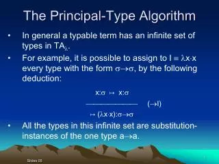
The Principal-Type Algorithm • In general a typable term has an infinite set of types in TA. • For example, it is possible to assign to I xx every type with the form , by the following deduction: x: ↦ x: (I) ↦ (xx): • All the types in this infinite set are substitution-instances of the one type aa. Slides 05
By the subject-construction theorem, every deduction for I must have the simple form shown before. • The type aa is called a principal type for I. • The existence of a principal type is a property of all typable terms, not just I. • The principal type of a term is the most general type it can receive in TA. • We shall learn that every typable term has a principal type. Slides 05
A principal-type (PT) or type-checking algorithm will decide whether a given term M is typable and, if the answer is "yes", will output a principal type for M. • The existence of a PT algorithm is what gives TA and its extensions such as Haskell and ML their practical value, since if the typability of a program is regarded as a safety criterion then the programmer will want to be able to decide effectively whether a newly created program satisfies this criterion. • In order to understand the PT algorithm, we need the knowledge of substitution and unification. Slides 05
Definition (3A1) A type-substitutions is any expression [1/a1, ..., n/an], where a1, ..., an are distinct type-variables and 1, ..., n are any types. For any we define s() to be the type obtained by simultaneously substituting 1 for a1, ..., n for an throughout . In more detail, we define • s(ai) i • s(b) b if b is an atom {a1, ..., an} • s() s()s(). We call s() an instance of . Slides 05
Example: Let s [(ab)/c] and (ab)(bc)ac, then s() (ab)(bab)aab. Slides 05
The case n = 0 is called the empty substitution, e. e() . • If n = 1, s will be called a single substitution. • Each part-expression i/ai of s will be called a component of s, and called trivial if i ai. • If all trivial components are deleted from s the resulting substitution will be called the nontrivial kernel of s. • {a1, ..., an}: Dom(s) Vars(1, ..., n): Range(s) Slides 05
Definition (3A2) The action of a substitution s is extended to finite sequences of types, to type-contexts and to TA-formulas, as follows: s(<1, ..., n>) = <s(1), ..., s(n)>, s() = {x1:s(1), ..., xm:s(m)} if = {x1:1, ..., xm:m}, s( ↦ M:) = s() ↦ M:s(). s() is the result of applying s to every TA-formula in deduction . Slides 05
Besides the concept of substitution s for type-variables just mentioned, we also have the concept of substitution for term-variables. • Lemma (2B6) Let 1 be consistent with 2 and let 1, x: ⊢M:, 2⊢N: then 1 2⊢ [N/x]M:. Slides 05
Definition (3A3) In TA, a principal type or PT of a term M is a type such that • ⊢M: for some , • if ' ⊢M: for some ' and , then is an instance of . • A PT of M completely characterizes the set of all types assignable to M. Slides 05
Example: aba is a PT of xyx • Is there a PT for xxx? Slides 05
Definition (3A4) A principal pair for a term M is a pair <,> such that the formula ↦ M: is TA-deducible and every other TA-deducible formula ' ↦ M: is an instance of ↦ M:. • Example: <,aba> is a principal pair for xyx. Slides 05
Definition (3A5) A principal deduction for a term M is a deduction of a formula ↦ M: such that every other deduction, whose conclusion's subject is M, is an instance of . To abbreviate "there exists a principal deduction of ↦ M:", we shall write ⊢pM:. • We will see that a typable term M has not only a most general type but also a deduction whose every step is most general. Slides 05
Principal-Type Theorem (3A6) Every typable term has a principal deduction and a principal type in TA. Further, there is an algorithm that will decide whether a given -term M is typable in TA, and if the answer is "yes", will output a principal deduction and principal type for M. Slides 05
More details on type-substitution • Definition (3B2) Substitutions s and t are extensionally equivalent (s =ext t ) iff s() t () for all . • Lemma (3B2.1) (i) b Dom(s) s(b) b. (ii) s =ext t iff s and t have the same non-trivial kernel. Slides 05
Definition (3B3) If s [1/a1, ..., n/an] and V is a given set of variables, the restriction s↾V of s to V is the substitution consisting of the components i/ai of s such that ai V. • Lemma (3B3.1) (s↾Vars())() s(). Slides 05
Definition (3B4) If s [1/a1, ..., n/an] and t [1/b1, ..., p/bp] and either a1, ..., an, b1, ..., bp are all distinct or ai bj i j, we define s t [1/a1, ..., n/an,1/b1, ..., p/bp] with repetitions omitted. • Lemma (3B4.1) (i) Dom(s t) = Dom(s ) Dom(t). (ii) If s =exts'andt =ext t'and s t is defined, then so is s' t'and s t =ext s' t'. Slides 05
The composition of two substitutions s and t is a simultaneous substitution that will have the same effect as applying t and s in succession. • Definition (3B5) If s and t are any substitutions, say s [1/a1, ..., n/an] and t [1/b1, ..., p/bp], we define s∘t [i1/ai1, ..., ih/aih, s(1)/b1, ..., s(p)/bp] where {ai1, ..., aih} = Dom(s)-Dom(t) and 0 h n. Slides 05
Example: s [(cd)/a,(ba)/b], t [(ba)/b] ab s(t ()) (cd)(ba)(cd) s∘t [(cd)/a,(s(ba))/b] [(cd)/a,((ba)(cd))/b] (s∘t)() (cd)(ba)(cd) But (s t )() s() (cd)ba Slides 05
[a/b] ∘ [b/a] ? ab ([a/b] ∘ [b/a])() ? [a/b]([b/a]()) ? Slides 05
Lemma (3B5.1) • Dom(s∘t) = Dom(s) ∪ Dom(t). • (s∘t)() s(t()). This also means an instance of an instance of is an instance of . • r∘(s∘t) =ext (r∘s)∘t. • s =ext s', t =ext t' s∘t =ext s'∘t'. Slides 05
The next lemma, which is important in the correctness proof of the PT algorithm, says that if a composition s∘t is extended to r (s∘t), the extended substitution can also be expressed as a composition with t, under certain conditions on r to prevent clashes. • Lemma (3B6:composition-extension) Let r, s, t be substitutions such that (i) Dom(r) (Dom(s)Dom(t)) = , (ii) Dom(r) Range(t) = . Then r (s∘t) and (r s)∘t are both defined and r (s∘t) (r s)∘t. Slides 05
Definition (3B7) A variables-for-variables substitution is a substitution s [b1/a1, ..., bn/an] where b1, ..., bn are variables (not necessarily distinct). If b1, ..., bn are distinct , s is called one-to-one, and if also {a1, ..., an} = Vars() for a given , s is called a renaming in . • Note: A one-to-one substitution may be a renaming in one type but not in another. For example, [b/a] is a renaming in aa but not in ab. Slides 05
Definition (3B8) We say is an alphabetic variant of , or and are identical modulo renaming, iff s() for some renaming s in . • Lemma (3B8.2: Uniqueness) Let be a principal type of a term M. Then is unique modulo renaming. Slides 05
Main ideas for the PT algorithm • The two main steps in the PT algorithm: • the computation of PT(xM) from PT(M), • the computation of PT(PQ) from PT(P) and PT(Q). • The first is easy, the second needs more work which is the core of the PT algorithm. Slides 05
Suppose we are trying to decide whether an application PQ is typable in TA, and we already know that PT(P) , PT(Q) . For simplicity suppose PQ has no free variables. Then the types assignable to P are generated from by substitution and those assignable to Q are generated from . Hence, if we can find substitutions s1 and s2 such that s1() s2(), we will be able to deduce a type for PQ by rule (E), as follows: ↦ P:s1()s1() ↦ Q:s2() (E) ↦ PQ:s1() Slides 05
Thus the problem of deciding whether PQ is typable reduces to that of finding substitutions s1 and s2 such that s1() s2(). • This suggests the next two definitions. Slides 05
Definition (3C2) (i) If s1() s2() we call a common instance (c.i.) of the pair <,>, and we call <s1,s2> a pair of converging substitutions for <,>. (ii) If <1, ..., n> s1(<1, ..., n>) s2(<1, ..., n>) we call <1, ..., n> a common instance of <1, ..., n> and <1, ..., n>. • Example: A c.i. of <a(bc),(ab)a> is the type (())(), and the corresponding converging substitutions are s1 [(())/a, /b, /c], s2 [()/a, /b]. Slides 05
Does every pair of types has a common instance? No. For example the pair <aa,(bb)b> has none. Slides 05
Definition (3C3) A most general common instance (m.g.c.i) of <,> is a common instance 0 such that every other common instance is an instance of 0. If 0 is an m.g.c.i. of <,> we call any pair <s1,s2> such that s1() s2() 0 an m.g.c.i.-generator for <,>. • M.g.c.i.'s are unique modulo renaming. Slides 05
Example: The pair <a(bc),(ab)a> has an m.g.c.i m0 (())(). Proof: Let a(bc), (ab)a. In slide 27 we have shown that m0 is a c.i. of and . To show that m0 is most general, let m be any other c.i., then we have m s1(a)(s1(b)s1(c)) (s2(a)s2(b))s2(a), which gives s1(a) s2(a)s2(b), s2(a) s1(b)s1(c). Therefore, s1(a) (s1(b)s1(c))s2(b) and m ((s1(b)s1(c))s2(b))(s1(b)s1(c)). Thus, m is an instance of m0. Slides 05
The problem of finding PT(PQ) reduces to that of finding an m.g.c.i of <,>. • We will need Robinson'sunification algorithm. Slides 05
Definition (3D1) (i) If there is a substitution s such that s() s() we say <,> is unifiable; we call any such s a unifier of <,> and call s() a unification of <,>. (ii) A unifier of a pair of sequences <<1, ..., n>, <1, ..., n>> is a substitution s such that s(<1, ..., n>) s(<1, ..., n>). Slides 05
Note: A unification of <,> is just a c.i. obtained by making the same substitution in as in . But not every c.i. is a unification. A pair <,> may have a c.i. but no unifier. For example, consider a(bc), (ab)a. We have seen in slide 27 that this pair has a c.i.; but no substitution s can exist such that s() s(), because this would imply s(a) s(a)s(b) which is impossible. Slides 05
Definition (3D2) A most general unifier (m.g.u.) of <,> is a unifier u such that for every other unifier s of <,> we have s() s'(u()) for some s'. If u() for some m.g.u. u of <,> we call a most general unification of <,>. • Lemma If u is an m.g.u. of <,> and v is a renaming of variables in u(), then v∘u is an m.g.u. of <,>. Slides 05
The m.g.u. of a pair <,> may differ from its m.g.c.i. However, in the special case that and have no common variables, every c.i. is also a unification. Why? Because if s1() s2() and Dom(s1) Vars() and Dom(s2) Vars() then s1 s2 is defined and (s1 s2)() (s1 s2)(). Slides 05
Lemma (3D3) (i) If and have no common variables, <,> has an m.g.u. iff it has an m.g.c.i., and the two are identical. (ii) For all and : if we change to an alphabetic variant * with no variables in common with , the unifications of <,*> will be exactly the common instances of <,> and the most general unification of <,*> will be the m.g.c.i. of <,>. • Thus the problem of finding m.g.c.i.'s has been reduced to that of finding most general unifications of pairs <,> with no variables in common. Slides 05
Unification Theorem (3D4) (i) There is an algorithm which decides whether a pair of types <,> has a unifier, and, if the answer is "yes", constructs its m.g.u. (ii) If a pair <,> has a unifier it has an m.g.u. (iii) Parts (i) and (ii) hold also for pairs of deductions and for pairs of finite type-sequences. Slides 05
Unification Algorithm (Robinson 1965) Input: any pair <,> of types. Output: either a correct statement that <,> is not unifiable or an m.g.u. u of <,>. Step 0. Choose k = 0 and u0 e (the empty substitution). Step k+1. Given k and uk, construct k uk() and k uk(), and apply the comparison procedure to <k,k>. That procedure will output either a correct statement that k k or a disagreement pair <a,> such that ≢ a. If k k, choose u uk. If k≢ k and the output of the comparison procedure is <a,>, decide whether a Vars(). If a Vars(), state that <,> is not unifiable and stop. If a Vars(), then replace k by k+1, choose uk+1 [/a]∘uk, and go to Step k+2. Slides 05
Comparison Procedure Given a pair <,> of types, write and as symbol-strings, say s1...sm, t1...tn (m, n 1) where each of s1, ..., sm, t1, ..., tn is an occurrence of a parenthesis, arrow or variable. If , then state that and stop. If ≢ , choose the least p Min{m,n} such that sp≢ tp. One of sp, tp must be a variable and the other must be a left parenthesis or a different variable. Further, sp is the leftmost symbol of a unique subtype * of . (If sp is a variable, * sp.) Similarly tp is the leftmost symbol of a unique subtype * of . Choose one of *, * that is a variable and call it "a". (If both are variables, choose the one that is first in the alphabet.) Then call the remaining member of <*,*> ""; the pair <a,> is called the disagreement pair for <,>. Slides 05
the PT algorithm Input: any -term M, closed or not. Output: either a principal deduction M for M or a correct statement that M is not typable. Case I. If M is a variable, say M x, choose M to be the one-formula deduction x:a↦ x:a, where a is any type-variable. Case II. If M xP and x FV(P), say FV(P) = {x, x1, ..., xt}, apply the algorithm to P. If P is not typable, neither is M. If P has a principal deduction P its conclusion must have the form x:, x1:1, ..., xt:t ↦ P: for some types , 1, ..., t, . Apply rule (I)main to make a deduction of x1:1, ..., xt:t ↦ (xP):. Call this deduction xP. Slides 05
Case III. If M xP and x FV(P), say FV(P) = {x1, ..., xt}, apply the algorithm to P. If P is not typable, neither is M. If P has a principal deduction P its conclusion must have the form x1:1, ..., xt:t ↦ P: for some types 1, ..., t, . Choose a new type-variable d not in P and apply (I)vac, vacuously discharging x:d, to get a deduction of x1:1, ..., xt:t ↦ (xP):d. Call this deduction xP. Slides 05
Case IV. If M PQ, apply the algorithm to P and Q. If P or Q is untypable then so is M. If P and Q are both typable, suppose they have principal deductions P and Q. First rename type-variables, if necessary, to ensure that P and Q have no common type-variables. Next list the free term-variables in P and those in Q (noting that these lists may overlap); say FV(P) = {u1, ..., up, w1, ..., wr} (p, r 0), FV(Q) = {v1, ..., vq, w1, ..., wr} (q 0), where u1, ..., up, v1, ..., vq, w1, ..., wr are distinct. Slides 05
Subcase IVa. M PQ and PT(P) is composite, say PT(P) . Then the conclusions of P and Q have the form, respectively, (1) u1:1, ..., up:p, w1:1, ..., wr:r ↦ P:, (2) v1:1, ..., vq:q, w1:1, ..., wr:r ↦ Q:. Apply the unification algorithm to the pair of sequences (3) <1, ..., r, >, <1, ..., r, >. Subcase IVa1. The pair (3) has no unifier. Then PQ is not typable. Slides 05
Subcase IVa2. The pair (3) has a unifier. Then the unification algorithm gives a most general unifier u; apply a renaming if necessary to ensure that (4) Dom(u) = Vars(1, ..., r, , 1, ..., r, ), (5) Range(u) V = , where (6) V = (Vars(P) Vars(Q)) – Dom(u). Then apply u to P and Q; this changes their conclusions to, respectively, u1:1*, ..., up:p*, w1:1*, ..., wr:r*↦ P:**, v1:1*, ..., vq:q*, w1:1*, ..., wr:r*↦ Q:*, where 1* u(1), etc. And by the definition of u we have 1* 1*, ..., r* r*, * *. Hence (E) can be applied to the conclusions of u(P) and u(Q). Call the resulting combined deduction PQ; its conclusion is (7) u1:1*, ..., up:p*, v1:1*, ..., vq:q*, w1:1*, ..., wr:r*↦ PQ:*. Slides 05
Subcase IVb. M PQ and PT(P) is atomic, say PT(P) b. Then the conclusions of P and Q have the form, respectively, (8) u1:1, ..., up:p, w1:1, ..., wr:r ↦ P:b, (9) v1:1, ..., vq:q, w1:1, ..., wr:r ↦ Q:. Choose any variable c Vars(P) Vars(Q) and apply the unification algorithm to the pair of sequences (10) <1, ..., r, b>, <1, ..., r, c>. Subcase IVb1. The pair (10) has no unifier. Then PQ is not typable. Slides 05
Subcase IVb2. The pair (10) has a unifier. Then the unification algorithm gives a most general unifier u; apply a renaming if necessary to ensure that (11) Dom(u) = Vars(1, ..., r, b, 1, ..., r, c), (12) Range(u) V = , where V = (Vars(P) Vars(Q)) – Dom(u). Then apply u to P and Q. By the definition of u, u(b) u(c) u()u(c), and thus the conclusions of u(P) and u(Q) are u1:1*, ..., up:p*, w1:1*, ..., wr:r*↦ P:*c*, v1:1*, ..., vq:q*, w1:1*, ..., wr:r*↦ Q:*, where * denotes application of the substitution u, and 1* 1*, ..., r* r*. Hence (E) can be applied to the conclusions of u(P) and u(Q). Call the resulting combined deduction PQ; its conclusion is u1:1*, ..., up:p*, v1:1*, ..., vq:q*, w1:1*, ..., wr:r*↦ PQ:c*. Slides 05
Theorem (3E3) The relation ⊢M: is decidable, i.e. there is an algorithm which accepts any M and and decides whether or not ⊢M:. Proof: Apply the PT algorithm to M. If M is not closed or not typable we cannot have ⊢M:. If M is closed and typable, decide whether is an instance of PT(M). Slides 05
Example: Apply the PT algorithm to check that the -term W xyxyy has the principal type (aab)ab. Slides 05