Download
1 / 39
390 likes | 522 Views
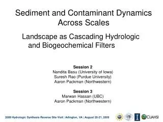
Sediment and Contaminant Dynamics Across Scales . Landscape as Cascading Hydrologic and Biogeochemical Filters. Session 2 Nandita Basu (University of Iowa) Suresh Rao (Purdue University) Aaron Packman (Northwestern) Session 3 Marwan Hassan (UBC) Aaron Packman (Northwestern).

E N D
Sediment and Contaminant Dynamics Across Scales Landscape as Cascading Hydrologic and Biogeochemical Filters Session 2 Nandita Basu (University of Iowa) Suresh Rao (Purdue University) Aaron Packman (Northwestern) Session 3 Marwan Hassan (UBC) Aaron Packman (Northwestern)
Conceptual Framework:Hierarchical, Non-linear Filters and Cascading Waves Reach Scale Hillslope Climate and Veg: Rain, ET Mgmt.: Chemical Inputs overland flow Source Release Model subsurface flow Water Column Vadose Zone : Storage, Transport Retardation, Transformations groundwater flow Saturated Zone : Transport, Retardation Transformations sediment Emergent Patterns
Approach: Pattern Based Patterns offer a window into landscape processes … and a starting point for hypotheses Hypotheses Testing: • WHAT are the “emergent” patterns? – Data • HOW are they created? – Models Hypotheses Generation: • WHEN will they cease to exist --- tipping points • Data-based (comparative hydrology) • Model-based
Patterns that Intrigued us….. Why are they linear? Or, Why are Watersheds Chemostatic? At what scale are they chemostatic? Nitrate load-discharge relationships across Mississippi Sediment load-discharge relationships
Motivating Questions: Can we understand the dominant classes of behavior of landscapes that will pave the way towards catchment biogeochemical classification? How are sediments and contaminants (dissolved and sediment bound) generated in the hillslope? How do sediments and contaminants get translated through the network?
Hypothesis: Landscapes act as cascading,coupled filters Observed “patterns” are windows into this filtering Filtering of variable inputs by landscape structure and biogeochemical processes produces PATTERNS, as water and solutes cascade across spatial and temporal scales
Four examples of solute filtering Event filtering in the vadose zone C vs Q: Data analysis across scales C vs Q: Models to understand controls Flow and denitrification in networks
HEIST: A 1-D event-based model of solute loads filtered by the vadose zone
Model reveals controls on clustering of events and emergence of extremes Effects of soil depth: Effects of degradation rate: Increasing degradation rates Increasing depth Solute mass out Solute mass in Clustering in time Increased non-linearity of filter “Extreme outcomes driven by normal inputs” Clustering of transported mass
Concentration vs Discharge: Data analysis across scales
Intra-annual filtering of nitrate more complex than less bioactive solutes in experimental watersheds Sulfate Sulfate Nitrate Nitrate Chloride Chloride Hubbard Brook WS2 Cumulative outputs over each year Cumulative oututs over each year Cumulative precipitation Cumulative discharge Complex filtering of Nitrate Simpler, but stronger filtering of less bioactive compounds
Flow and Nitrate decouple at larger spatial scales, except for specific events, in a data-rich agricultural watershed Single tile drain (0.03 km2) Q-C strongly coupled Watershed (186 km2) Episodically coupled Flow vs Nitrate coherence analysis on 10 years of daily data
Landuse and climate control mean [N], and interannual variability is dampened, at Mississippi watershed scale Annual NO2 + NO3 Load (t/km2/yr) Annual Discharge 106 m3/km2/yr At larger scales, inter-anual variability in concentration is dampened Average concentration influenced by climate + land-use + ...
Concentration vs Discharge: Models to understand controls
Multiple models used to test hypotheses about origins of observed patterns MRF model - Conceptual hillslope coupled to network THREW model - Representative Elementary Watershed Storage-dependent CSTR model Multi-compartment flow and BGC process model Storage
Chemostatic Q – C behavior linked to: B) Interaction of forcing and filter timescales A) Storage – dependentreaction rates Reaction time Residence time Event input frequency C) Averaging effects of the network
Reach scale dependence on stage shown to produce intriguing patterns when up-scaled in time and space Simon Donner (UBC) IBIS-THMB model simulations (65 sq km grid resolution) Bohlke 2008 k = 0.06/h In-stream N Removal Temporal averagingover year Spatial averaging over network Runoff (mm) REACH SCALE Inverse relationship between denitrification and stream depth k = 0.2/h
Order from complexity • Solute filtering behavior most complex at • small scales • more bioactive solutes • Critical control on filtering: • Coupling of flow and reaction rates • Timescales of forcing, processing • Spatial structure of the network • Models built around event filtering can reproduce patterns of • Episodic leaching • Nitrate concentration vs discharge • Denitrification across scales
Study Sites Rio Isabena, Spain Goodwin Creek, Mississippi
Landscape and Network Filtering of Sediment Transport Rainfall Bank Erosion Land Management Runoff, Suspended Sediment Deposition and Resuspension Cuml. Load Q(t) Cuml. Flow
Hillslope Filtering Precipitation Deviations from the Mean (mm) Flow Sediment Mobilized 1982 1997 Years Deviations from the Mean (kg) Deviations from the Mean (m) 1997 1982 1997 1982 Years Years
Hillslope Filtering Precipitation Deviations from the Mean (mm) Flow ~ unfiltered precipitation Flow Sediment Mobilized 1982 1997 Years Deviations from the Mean (kg) Deviations from the Mean (m) 1997 1982 1997 1982 Years Years
Hillslope Filtering Precipitation Deviations from the Mean (mm) Sediment ~ flow filtered Flow Sediment Mobilized 1982 1997 Years Deviations from the Mean (kg) Deviations from the Mean (m) 1997 1982 1997 1982 Years Years
Hillslope Filtering Precipitation Deviations from the Mean (mm) Sediment ~ flow filtered Flow Sediment Mobilized 1982 1997 Years Deviations from the Mean (kg) Deviations from the Mean (m) Increased Disturbance 1997 1982 1997 1982 Years Years
1982 1983 1984 1985 1986 1987 1988 1989 EXCEEDENCE PROBABILITY 1990 1991 1992 1993 1994 1995 1996 1997 NORMALIZED FLOW AND LOAD Hillslope Filtering – Land Use FLOW LOAD CHANGE IN LANDUSE
Quantification of Bank Erosion 1997/3/4 1996/12/9 1996/4/24
Sediment Transport – Waves INPUT Concentration Flow Sediment Concentration in Bed Length Down Reach (m)
Sediment Transport – Waves INPUT Concentration Flow Sediment Concentration in Bed Length Down Reach (m)
Sediment Transport – Waves INPUT Concentration Flow Sediment Concentration in Bed Length Down Reach (m)
Sediment Transport – Waves INPUT Concentration Flow Sediment Concentration in Bed Length Down Reach (m)
Sediment transport behaviour • Reproduces features of export patterns
Basin-Scale Filtering Land Use Intervention Load – relatively homogeneous Load – highlights channel contributions
Consequences • Intact ecosystems more filtering • Network has “memory” • Responses vary in space, time • Filtering: • Nonlinear (e.g. hillslopes) • Episodic (e.g. legacy) • Stochastic (e.g. bank failure)
Order out of Complexity Catchment Scale: Nutrient Increasing depth Solute mass out Vadose Zone Solute mass in Network Scale Sediment