Download

1 / 27
290 likes | 381 Views
Risk Attitude. Dr. Yan Liu Department of Biomedical, Industrial & Human Factors Engineering Wright State University. Payoff. (0.5). $30. Game 1. (0.5). -$1. (0.5). $2,000. Game 2. (0.5). -$1,900. Introduction.

E N D
Risk Attitude Dr. Yan Liu Department of Biomedical, Industrial & Human Factors Engineering Wright State University
Payoff (0.5) $30 Game 1 (0.5) -$1 (0.5) $2,000 Game 2 (0.5) -$1,900 Introduction This example illustrates that EMV analysis does not capture risk attitudes of decision makers. Individuals who are afraid of risk or are sensitive to risk are called risk-averse. EMV=$14.5 Which game would you choose, game 1 or game 2? EMV=$50 If EMV is the basis for the decision, you should choose Game 2. Most of us, however, may consider Game 2 to be too risky and thus choose Game 1.
Utility U(x) Dollars x Utility Function • Utility functions are models of an individual’s attitude toward risk • Utility functions translate dollars into utility units • Graph • Table • Mathematical expression A utility function that displays risk-aversion (upward sloping and concave)
Risk Attitude • Risk-Averse: Afraid or Sensitive to Risk • Would trade a gamble for a sure amount that is less than the expected value of the gamble • U(x) is a concave curve (continuous) (discrete) • Risk-Seeking: Willing to Accept More Risk • Would play a state lottery • U(x) is a convex curve (continuous) (discrete) • Risk-Neutral: An EMV Decision Maker • Maximizing utility is the same as maximizing EMV • U(x) is a straight line is constant (continuous) (discrete)
Utility Risk-Neutral Risk-Seeking Risk-Averse Dollars Risk Attitude (Cont.) Shapes of Utility Functions of Three Different Risk Attitudes
Some Terminologies • Expected Utility (EU) • Weighted average of utilities of all possible states • Certainty equivalent (CE) • Amount of money equivalent to the situation that involves uncertainty • Risk Premium • Difference between the EMV and the CE, i.e., the amount you would pay to avoid the risk You have a lottery which has 0.3 probability of winning $200 and 0.7 probability of losing $10, and you are willing to sell it for $30. Your certainty equivalent for this lottery is $30 The risk premium of the lottery is: (0.3*200+0.7*(-10))-30 =53-30=$23
Utility Utility Curve U(CE) = EU Expected Utility (EU) Risk Premium Certainty Equivalent (CE) EMV Dollar Graphical Representation of Expected Utility, Certainty Equivalent, and Risk Premium For a risk-seeking person, CE would be on the right side of EMV on the horizontal axis
Utility Assessment • Assessing a Utility Function is a Subjective Judgment • Different people have different risk attitudes toward risk and are willing to accept different levels of risk • Two Methods • Assessment using certainty equivalent • Assessment using probabilities
Utility Function Assessment Via Certainty Equivalence • Assess several certainty equivalents from which the utility function is derived • Step 1: set the utility of the best payoff to 1 and the utility of the worst payoff to 0 • Step 2: Construct a situation that involves uncertainty and find its CE using reference lottery. • Step 3: Calculate the expected utility of the lottery, EU. Because EU is equal to U(CE), we get another point (CE, EU) on the utility curve • Step 3: Repeat Steps 2 and 3 until getting enough points to plot the utility curve
You face an uncertain situation in which you may earn $10 in the worst case, $100 in the best case, or some amount in between. You have a variety of options, each of which leads to some uncertain payoff between $10 and $100. To evaluate the alternatives, you must assess your utility for payoffs from $10 to $100. • Step 1: let U(10)=0 and U(100)=1 • Step 2: imagine you have the opportunity to play the following reference lottery (0.5) $100 A (0.5) Suppose your CE in this lottery is $30 $10 B CE • Step 3: Calculate EU of lottery A, which is 0.5∙U(100)+0.5∙U(10)=0.5. Therefore, U(30)=0.5 and you have found a third point on your utility curve. • Step 4: To find another point, you can take a different reference lottery, say using $100 and $30 as two equally likely outcomes in lottery A, and then follow steps 2 and 3. Continue with the same procedures until you have enough points to plot the utility function.
U(x) x (Dollars) Suppose you now have five points on your utility curves: U(10)=0, U(18)=0.25, U(30)=0.5, U(50)=0.75, and U(100)=1, you can plot the utility function
(p) $100 C (1-p) $10 $65 D U(65) = p∙U(100) + (1-p)∙U(10) = p∙1+(1-p)∙0 = p Utility Function Assessment Via Probability-Equivalent • Assess the utility of a selected dollar amount directly • Adjust the probability in the reference lottery
Gambles, Lotteries, and Investments • Framing utility assessment in terms of gambles or lotteries may evoke images of carnival games or gambling which seem irrelevant to decision making or even distasteful • An alternative is to think in terms of risky investment, particularly for investment decisions • Whether you should make a particular investment
Risk Tolerance and Exponential Utility Function • Exponential Utility Function R is risk tolerance, showing how risk-adverse the function is. Larger R means less risk-adversion and makes the utility function flatter Exponential Utility Functions with Three Different Risk Tolerances x ↑ => U(x) →1 x =0 => U(x) = 0
Risk Tolerance and Exponential Utility Function (Cont.) • Assess Risk Tolerance R (0.5) $Y E (0.5) – $Y/2 F $0 The largest Y for which you prefer to take gamble E is approximately equal to your risk tolerance Suppose you decide Y is $900, then R=900, and your utility function is
Risk Tolerance and Exponential Utility Function (Cont.) • Find CE of Given Uncertain Event • First calculate the expected utility (EU) of the uncertain event • Since U(CE)=EU, you can solve the equation to get CE • If you estimate the expected value, ,and variance, , of the payoffs, then CE can be approximately calculated as
The expected utility of the gamble is: EU = 0.4∙U($2000)+0.4 ∙U($1000)+ 0.2∙U($500) = 0.4∙(1-e-2000/900) +0.4 ∙(1-e-1000/900)+ 0.2∙(1-e1-500/900) = 0.710 Solve 0.710=1-e-CE/900 for CE, you can get CE=$1114.71 Suppose you face the following gamble: 1) win $2000 with probability 0.4; 2) win $1000 with probability 0.4, or 3) win $500 with probability 0.2, and your utility can be modeled as an exponential function with R=900. What is your CE of this gamble?
Constant and Decreasing Risk-Aversion • Constant Risk-Aversion • The risk premium for a gamble does not depend on the initial wealth held, • Can be represented using an exponential utility function You have $x in your pocket, and you are facing a bet: 1) win $15 with probability 0.5, or 2) lose $15 with probability 0.5. Suppose your utility function can be modeled as an exponential function with risk tolerance R=35. $ in Pocket (0.5) $x+15 (0.5) $x –15 Probability Tree of the Bet
When x=$25 EU=0.5∙U($10)+0.5∙U($40)=0.5∙(1-e-10/35)+0.5∙(1-e-40/35)=0.4648 EU=U(CE) 0.4648=1-e-CE/35CE=$21.88 EMV= 0.5∙10+0.5∙40=$25 Risk Premium=EMV-CE=25-21.88=$3.12
Constant and Decreasing Risk-Aversion (Cont.) • Decreasing Risk-Aversion • Typically, people’s attitude towards risk changes with their initial wealth • The risk premium for a gamble decreases along with the increase of wealth held • Can be represented with the logarithmic utility function
In the previous example of betting, suppose your utility function can be modeled as a logarithmic function When x=$25 EU=0.5∙U($10)+0.5∙U($40)=0.5∙ln(10)+0.5∙ln(40)=2.9957 EU=U(CE) 2.9957=ln(CE)CE=$20 EMV= 0.5∙10+0.5∙40=$25 Risk Premium=EMV-CE=25-20=$5
Some Caveats • Utilities DO NOT Add Up • U(A+B)≠U(A)+U(B) (why?) • Utility Difference Does Not Express Strength of Preferences • U(A1)-U(A2) > U(B1)-U(B2) does not mean we would rather go from A1 to A2 instead of from B1 to B2 • Utility only provides a numerical scale for ordering preferences, not a measure of their strengths • Utilities are Not Comparable from Person to Person • A utility function is a subjective personal statement of an individual’s preference
Exercise • An investor with assets of $10,000 has an opportunity to invest $5,000 in a venture that is equally likely to pay either $15,000 or nothing. The investor’s utility function can be described by the log utility function U(x) =ln(x), where x is the total wealth. • What should the investor do?
Total Wealth success (0.5) 10,000-5,000+15,000 =$20,000 $15,000 Failure (0.5) 10,000-5,000= $5,000 Invest - $5,000 Don’t Invest $10,000 a. EU(invest) = 0.5∙U($20,000)+0.5∙U($5,000)=0.5∙ln($20,000)+0.5∙ln($5000) = 9.21 EU(Don’t invest) = U($10,000) = ln($10,000) = 9.21 Therefore, the investor is indifferent between the two alternatives
b. Suppose the investor places a bet with a friend before making the investment decision. The bet is for $1,000; if a fair coin lands heads up, the investor wins $1,000, but if it lands tails up, the investor pays $1,000 to his friend. Only after the bet has been resolved will the investor decide whether or not to invest in the venture. If he wins the bet, should he invest? What if he loses the bet? Should he toss the coin in the first place?
b. EU(Invest|Win) = 9.326 Total Wealth Success (0.5) 10,000+1,000-5,000+15,000 =$21,000 $15,000 Invest Failure (0.5) 10,000+1,000-5,000= $6,000 Win (0.5) -$5,000 EU(Don’t Invest|Win) = 9.306 $1,000 Don’t Invest 10,000+1,000= $11,000 Success (0.5) EU(Bet) = 9.216 10,000-1,000-5,000+15,000 =$19,000 EU(Invest|Lose) = 9.073 $15,000 Invest Failure (0.5) Bet 10,000-1,000-5,000= $4,000 Lose (0.5) -$5,000 -$1,000 Don’t Invest EU(Don’t Invest|Lose) = 9.105 10,000-1,000 = $9,000 Don’t Bet Success (0.5) 10,000-5,000+15,000 =$20,000 $15,000 Invest EU(Don’t Bet) = 9.21 Failure (0.5) 10,000-5,000= $5,000 -$5,000 Don’t Invest $10,000
If he wins the bet: EU(Invest) = 0.5∙ln($21,000) + 0.5∙ln($6,000) = 9.326 EU(Don’t Invest) = ln($11,000) = 9.306 Therefore, if he wins the bet, he should invest the venture If he loses the bet: EU(Invest) = 0.5∙ln($19,000) + 0.5∙ln($4,000) = 9.073 EU(Don’t Invest) = ln($9,000) = 9.105 Therefore, if he losses the bet, he should not invest the venture EU(Bet) = 0.5∙EU(Invest|win) + 0.5∙EU(Don’t Invest |lose) = 0.5(9.326)+0.5(9.105) = 9.216 EU(Don’t Bet) = 9.21 (from part a) Therefore, he should bet