Final Review

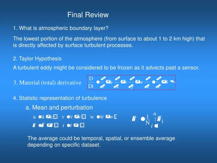
1. Final Review 1. What is atmospheric boundary layer? The lowest portion of the atmosphere (from surface to about 1 to 2 km high) that is directly affected by surface turbulent processes. 2. Taylor Hypothesis A turbulent eddy might be considered to be frozen as it advects past a sensor. 3. Material (total) derivative 4. Statistic representation of turbulence a. Mean and perturbation The average could be temporal, spatial, or ensemble average depending on specific dataset.

2. b. Reynolds average covariance variance Standard deviation Correlation coefficient c. Turbulent kinetic energy (TKE) 5. Turbulent flux a. Sensible heat flux, Latent heat flux, buoyancy flux Sensible heat flux, SH

3. Latent heat flux, LE Buoyancy flux, Momentum flux, MO Z b. Reynolds stress V Tensor X

4. 6. Frictional velocity 7. Mean governing equations in turbulent flow

5. 8 TKE budget equation A. Local change term D. Buoyancy production term E. Transport term B. Advection term C. Shear production term F. Pressure correlation term G. Dissipation For horizontal homogeneous condition, x direction along the mean wind direction, mean vertical velocity is zero.

6. 9. Static stability and instability The atmosphere is unstable if a parcel at equilibrium is displaced slightly upward and finds itself warmer than its environment and therefore continues to rise spontaneously away from its starting equilibrium point. The atmosphere is stable if a parcel at equilibrium is displaced slightly upward and finds itself colder than its environment andtherefore sink back to its original equilibrium point. Stable Unstable 10. Thermodynamic structure of atmospheric boundary layer

7. 11. Richardson number a. Flux Richardson number b. Gradient Richardson number Turbulent flow Non-turbulent flow c. Bulk Richardson number

8. 12. Turbulent closure problem Simplified governing equations a. First-order closure Z

9. 13. Monin-Obukhov length L Static unstable Dynamic unstable Static stable Dynamic stable Using surface layer relation Static unstable Dynamic unstable Static stable Dynamic stable

10. 14. Turbulent Analyses a. Fourier Transform Why do we need the frequency information? No frequency information is available in the time-domain signal!

11. b. Discrete Fourier Transform Observations: N Sampling interval: Period First harmonic frequency: All frequency: nth harmonic frequency: c. Aliasing, Nyquist frequency, and folding If sampling rate is , the highest wave frequency can be resolved is , which is called Nyquist frequency

12. example If there were a true signal of f=0.9 Hz that was sampled at fs=1.0 Hz, then, one would find that the signal has been interpreted as the signal of f=0.1 Hz. In other words, the real signal f=0.9 Hz was folded into the signal f=0.1Hz. Folding occurs at Nyquist frequency. What problem does folding cause?

13. d. Leakage

14. e. Detrend, window

15. f. Energy Spectrum Discrete spectral intensity (or energy) g. Spectral energy density h. Turbulent energy cascade Turbulent spectral similarity • Energy associated with large-scale motion • eventually is transferred to the large • turbulent eddies. • The large eddies then transport this energy • to small-scale eddies. • These smaller scale eddies then transfer • the energy to even small-scale eddies..., • and so on • Eventually, the energy is dissipated into • heat via molecular viscosity.

16. I. Kolmogorov's Energy Spectrum Inertial sub-range is in an equilibrium state, Kolmogorov assumes that the energy density per unit wave number depends only on the wave number and the rate of energy dissipation. wavelength wave-number 3 3 5 5

17. 16. Ekman Spiral in the atmospheric boundary layer Boundary conditions Ekman layer. Atmosphere:

18. Boundary layer vertical secondary circulation divergence convection D convergence Hurricane Dynamics of vortex spin down and spin up

19. 17. Oceanic Ekman layer Boundary condition: Solution:

20. 18. Application of Pi theory in the surface How to represent in terms of relevant parameters: Four variables and two basic units result in two dimensionless numbers, e.g.: The standard way of formulating this is by defining: Monin-Oubkhov length

21. 19. Similarity theory a. Neutral condition b. Non-neutral condition

22. Temperature profiles in the surface layer Similarly,

23. 20. Bulk transfer relations Drag coefficient of momentum, heat, and moisture.

24. 19. Flux footprint Flux footprint describes a dependence of vertical turbulent fluxes, such as, heat, water, gas, and momentum transport, onthe condition of upwind area seen by the Instruments. Another frequently used term representing the same concept is fetch. 20. The surface energy balance atmosphere SH LE Land or Ocean Difference between heat capacity and specific heat.

25. Diurnal variation of surface energy budget over land Wet surface Dry surface Radiative heating at the surface

26. 21. Convective Boundary Layer Turbulent Potential temperature (K) Buoyancy fluxes (K m/s)

27. Mixed layer model subsidence h CBLGrowth Entrainment warming Entrainment drying turbulence MixedLayer 1. ML warming caused by heat input from the surface and entrainment 2. Growth of the CBL controlled by entrainment and subsidence 3. ML moistening or drying due to surface evaporation and entrainment

28. Some important relations under the mixed layer model framework h Deardorff convective velocity scale or Mixed layer depth Surface buoyancy flux Empirical relations in the mixed layer

29. 22. Convective plume structures, skewness, and Kurtosis Narrow branch of updraft compensated by broad branch of downdraft Skewed distribution Skewness Kurtosis

30. 23. Nocturnal boundary layer

31. Nocturnal jet: Nocturnal jet forms at night-time overland under clear sky conditions. The wind speed may be significantly super-geostrophic.

32. Inertial oscillation theory Governing equations Further assuming daytime boundary layer is in a steady state After sunset, nocturnal boundary layer forms, the air above the NBL can be assumed to be free atmosphere, the governing equation becomes It has a solution in the format of

33. Initial condition Solution 2 3 1 4 0 5 6 15 7 14 8 13 9 12 10 11 Influence of slope z

34. 24. Inflection-point instability in rotation-shear flow Barotropic Ekman flow with constant Km (the simplest PBL flow) y Vg x v u ξ×1000 Roll axis z ξ Inflection point Vorticity maximum ε

35. In the roll-coordinate, the vorticity equation of horizontal homogeneous Boussinesq flow Procedure for solving the problem (classic linear method) 1. Using small perturbation method to linearize equation 2. Assuming simple harmonic wave solution m is the wavenumber; c is the complex eigenvalue with real part the wave velocity and imaginary part the growth rate. 3. Obtaining Rayleigh necessary condition for instability

36. Wavenumber m The maximum growth rate of 0.028 occurs at wavenumber 0.5 and oriented 18o to the left of the geostrophic wind.(Brown 1972 JAS)

37. 25. Boundary layer clouds St & Sc St & Sc subsidence Trade wind inversion Stratus and stratocumulus Transition Trade cumulus Intertropiccal Convergence Zone (ITCZ)

38. SW cloud forcing = clear-sky SW radiation – full-sky SW radiation LW cloud forcing = clear-sky LW radiation – full-sky LW radiation Net cloud forcing (CRF) = SW cloud forcing + LW cloud forcing Cloud radiative effects depend on cloud distribution, height, and optical properties. Low cloud High cloud SW cloud forcing dominates LW cloud forcing dominates

39. In GCMs, clouds are not resolved and have to be parameterized empirically in terms of resolved variables. water vapor (WV) cloud surface albedo lapse rate (LR) WV+LR ALL

40. Aerosol feedback Direct aerosol effect: scattering, reflecting, and absorbing solar radiation by particles. Primary indirect aerosol effect (Primary Twomey effect): cloud reflectivity is enhanced due to the increased concentrations of cloud droplets caused by anthropogenic cloud condensation nuclei (CNN). Secondary indirect aerosol effect (Second Twomey effect): 1. Greater concentrations of smaller droplets in polluted clouds reduce cloud precipitation efficiency by restricting coalescence and result in increased cloud cover, thicknesses, and lifetime.

41. Mechanisms of maintaining cloud-topped boundary layer • Surface forcing • Cloud top radiative cooling • Cloud top evaporative cooling