Download
1 / 119
1.2k likes | 1.36k Views
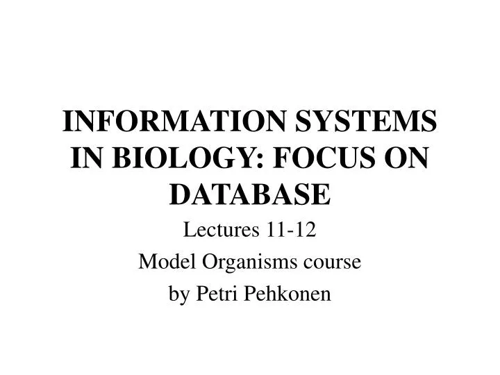
INFORMATION SYSTEMS IN BIOLOGY: FOCUS ON DATABASE. Lectures 11-12 Model Organisms course by Petri Pehkonen. Lecture contents. Theory of databases and information systems Biological databases Model organism databases. Information system architectures. Theory of databases.

E N D
INFORMATION SYSTEMS IN BIOLOGY: FOCUS ON DATABASE Lectures 11-12 Model Organisms course by Petri Pehkonen
Lecture contents • Theory of databases and information systems • Biological databases • Model organism databases
Theory of databases • Book: Database System Concepts • Available also in University library • Slides for this part modified from book Web material at http://codex.cs.yale.edu/avi/db-book/slide-dir/
Database Management System (DBMS) • DBMS contains information about a particular enterprise • Collection of interrelated data • Set of programs to access the data • An environment that is both convenient and efficient to use • Database Applications: • Banking: all transactions • Airlines: reservations, schedules • Universities: registration, grades • Sales: customers, products, purchases • Online retailers: order tracking, customized recommendations • Manufacturing: production, inventory, orders, supply chain • Human resources: employee records, salaries, tax deductions • Databases touch all aspects of our lives
Purpose of Database Systems • In the early days, database applications were built directly on top of file systems • Drawbacks of using file systems to store data: • Data redundancy and inconsistency • Multiple file formats, duplication of information in different files • Difficulty in accessing data • Need to write a new program to carry out each new task • Data isolation — multiple files and formats • Integrity problems • Integrity constraints (e.g. account balance > 0) become “buried” in program code rather than being stated explicitly • Hard to add new constraints or change existing ones
Purpose of Database Systems (Cont.) • Drawbacks of using file systems (cont.) • Atomicity of updates • Failures may leave database in an inconsistent state with partial updates carried out • Example: Transfer of funds from one account to another should either complete or not happen at all • Concurrent access by multiple users • Concurrent accessed needed for performance • Uncontrolled concurrent accesses can lead to inconsistencies • Example: Two people reading a balance and updating it at the same time • Security problems • Hard to provide user access to some, but not all, data • Database systems offer solutions to all the above problems
Examples of DBMS • MySQL • Free-to-use open source database • Efficient • Relational data model • SQL query language • Posgress • Free-to-use • Object oriented data model • SQL • AceDB • Free database system developed for data mining purposes of biosciences • AQL query language • Oracle • Commercial database system • Very efficient data processing • Optimization features for advanced data mining tasks
Data Models • A collection of tools for describing • Data • Data relationships • Data semantics • Data constraints • Relational model • Entity-Relationship data model (mainly for database design) • Object-based data models (Object-oriented and Object-relational) • Semistructured data model (XML) • Other older models: • Network model • Hierarchical model
The most popular: Relational Database • A relational database is based on the relational data model • Data and relationships among the data is represented by a collection of tables • Includes Data Manipulation Language (DML) and Data Definition Language (DDL) for searching and updating database • Most commercial relational database systems employ the SQL query langue
Relational Model Attributes • Example of tabular data in the relational model
Attribute Types • Each attribute of a relation has a name • The set of allowed values for each attribute is called the domain of the attribute • Attribute values are (normally) required to be atomic; that is, indivisible • E.g. the value of an attribute can be an account number, but cannot be a set of account numbers • Domain is said to be atomic if all its members are atomic • The special value null is a member of every domain • The null value causes complications in the definition of many operations • We shall ignore the effect of null values in our main presentation and consider their effect later
Relation Schema • A1, A2, …, Anare attributes • R = (A1, A2, …, An ) is a relation schema Example: Customer_schema = (customer_name, customer_street, customer_city) • r(R) denotes a relationr on the relation schema R Example: customer (Customer_schema)
Relation Instance • The current values (relation instance) of a relation are specified by a table • An element t of r is a tuple, represented by a row in a table attributes (or columns) customer_name customer_street customer_city Jones Smith Curry Lindsay Main North North Park Harrison Rye Rye Pittsfield tuples (or rows) customer
Database • A database consists of multiple relations • Information about an enterprise is broken up into parts, with each relation storing one part of the information account : stores information about accountsdepositor : stores information about which customer owns which account customer : stores information about customers • Storing all information as a single relation such as bank(account_number, balance, customer_name, ..)results in • repetition of information • e.g.,if two customers own an account (What gets repeated?) • the need for null values • e.g., to represent a customer without an account • Normalization theory (Chapter 7) deals with how to design relational schemas
Keys * • Attributes with unique contents • Identify the tuples * * *
Foreign Keys • A relation schema may have an attribute that corresponds to the primary key of another relation. The attribute is called a foreign key. • E.g. customer_name and account_number attributes of depositor are foreign keys to customer and account respectively. • Only values occurring in the primary key attribute of the referenced relation may occur in the foreign key attribute of the referencing relation. • Schema diagram
Relational Algebra • Procedural language • Six basic operators • select: • project: • union: • set difference: – • Cartesian product: x • rename: • The operators take one or two relations as inputs and produce a new relation as a result.
Select Operation – Example • Relation r A B C D 1 5 12 23 7 7 3 10 • A=B ^ D > 5(r) A B C D 1 23 7 10
Union Operation – Example • Relations r, s: A B A B 1 2 1 2 3 s r A B 1 2 1 3 • r s:
Aggregate Functions and Operations • Aggregation function takes a collection of values and returns a single value as a result. avg: average valuemin: minimum valuemax: maximum valuesum: sum of valuescount: number of values • Aggregate operation in relational algebra E is any relational-algebra expression • G1, G2 …, Gn is a list of attributes on which to group (can be empty) • Each Fiis an aggregate function • Each Aiis an attribute name
Aggregate Operation – Example • Relation r: A B C 7 7 3 10 • gsum(c) (r) sum(c ) 27
Modification of the Database • The content of the database may be modified using the following operations: • Deletion • Insertion • Updating • All these operations are expressed using the assignment operator of relational algebra
How to use relational algebra in practice: SQL • SQL: widely used non-procedural language • Example: Find the name of the customer with customer-id 192-83-7465select customer.customer_namefrom customerwherecustomer.customer_id = ‘192-83-7465’ • Example: Find the balances of all accounts held by the customer with customer-id 192-83-7465selectaccount.balancefromdepositor, accountwheredepositor.customer_id = ‘192-83-7465’ anddepositor.account_number = account.account_number • Application programs generally access databases through one of • Language extensions to allow embedded SQL • Application program interface (e.g., ODBC/JDBC) which allow SQL queries to be sent to a database
The select Clause • The select clause list the attributes desired in the result of a query • corresponds to the projection operation of the relational algebra • Example: find the names of all branches in the loan relation:select branch_namefrom loan • In the relational algebra, the query would be: branch_name (loan) • NOTE: SQL names are case insensitive (i.e., you may use upper- or lower-case letters.) • E.g. Branch_Name ≡ BRANCH_NAME ≡ branch_name • Some people use upper case wherever we use bold font.
The where Clause • The whereclause specifies conditions that the result must satisfy • Corresponds to the selection predicate of the relational algebra. • To find all loan number for loans made at the Perryridge branch with loan amounts greater than $1200. select loan_numberfrom loanwhere branch_name ='Perryridge'and amount > 1200 • Comparison results can be combined using the logical connectives and, or, and not. • Comparisons can be applied to results of arithmetic expressions.
The from Clause • The fromclause lists the relations involved in the query • Corresponds to the Cartesian product operation of the relational algebra. • Find the Cartesian product borrower X loan select from borrower, loan • Find the name, loan number and loan amount of all customers having a loan at the Perryridge branch. select customer_name, borrower.loan_number, amountfrom borrower, loanwhere borrower.loan_number = loan.loan_number andbranch_name = 'Perryridge'
String Operations • SQL includes a string-matching operator for comparisons on character strings. The operator “like” uses patterns that are described using two special characters: • percent (%). The % character matches any substring. • underscore (_). The _ character matches any character. • Find the names of all customers whose street includes the substring “Main”. select customer_namefrom customerwherecustomer_street like '% Main%' • Match the name “Main%” like 'Main\%' escape '\' • SQL supports a variety of string operations such as • concatenation (using “||”) • converting from upper to lower case (and vice versa) • finding string length, extracting substrings, etc.
Set Operations • Find all customers who have a loan, an account, or both: (selectcustomer_name from depositor)union(selectcustomer_name from borrower) • Find all customers who have both a loan and an account. (selectcustomer_name from depositor)intersect(selectcustomer_name from borrower) • Find all customers who have an account but no loan. (selectcustomer_name from depositor)except(selectcustomer_name from borrower)
Aggregate Functions • Find the average account balance at the Perryridge branch. select avg (balance)from accountwhere branch_name = 'Perryridge' • Find the number of tuples in the customer relation. select count (*)from customer • Find the number of depositors in the bank. select count (distinct customer_name)from depositor
Modification of the Database – Insertion • Add a new tuple to account insert into accountvalues ('A-9732', 'Perryridge', 1200) or equivalentlyinsert into account (branch_name, balance, account_number)values ('Perryridge', 1200, 'A-9732') • Add a new tuple to account with balance set to null insert into accountvalues ('A-777','Perryridge', null )
Joined Relations** • Join operations take two relations and return as a result another relation. • These additional operations are typically used as subquery expressions in the from clause • Join condition – defines which tuples in the two relations match, and what attributes are present in the result of the join. • Join type – defines how tuples in each relation that do not match any tuple in the other relation (based on the join condition) are treated.
Joined Relations – Datasets for Examples • Relation loan • Relation borrower • Note: borrower information missing for L-260 and loan information missing for L-155
Joined Relations – Examples • loan inner join borrower onloan.loan_number = borrower.loan_number • loan left outer join borrower onloan.loan_number = borrower.loan_number
Database Design The process of designing the general structure of the database: • Logical Design – Deciding on the database schema. Database design requires that we find a “good” collection of relation schemas. • Business decision – What attributes should we record in the database? • Computer Science decision – What relation schemas should we have and how should the attributes be distributed among the various relation schemas? • Physical Design – Deciding on the physical layout of the database
Modeling • A database can be modeled as: • a collection of entities, • relationship among entities. • An entityis an object that exists and is distinguishable from other objects. • Example: specific person, company, event, plant • Entities have attributes • Example: people have names and addresses • An entity set is a set of entities of the same type that share the same properties. • Example: set of all persons, companies, trees, holidays
Entity Sets customer and loan customer_id customer_ customer_ customer_ loan_ amount name street city number
Relationship Sets • A relationship is an association among several entities Example:HayesdepositorA-102customer entity relationship set account entity • A relationship set is a mathematical relation among n 2 entities, each taken from entity sets {(e1, e2, … en) | e1 E1, e2 E2, …, en En}where (e1, e2, …, en) is a relationship • Example: (Hayes, A-102) depositor
Attributes • An entity is represented by a set of attributes, that is descriptive properties possessed by all members of an entity set. • Domain – the set of permitted values for each attribute • Attribute types: • Simple and composite attributes. • Single-valued and multi-valued attributes • Example: multivalued attribute: phone_numbers • Derived attributes • Can be computed from other attributes • Example: age, given date_of_birth Example: customer = (customer_id, customer_name, customer_street, customer_city ) loan = (loan_number, amount )
Mapping Cardinality Constraints • Express the number of entities to which another entity can be associated via a relationship set. • Most useful in describing binary relationship sets. • For a binary relationship set the mapping cardinality must be one of the following types: • One to one • One to many • Many to one • Many to many
Mapping Cardinalities One to one One to many Note: Some elements in A and B may not be mapped to any elements in the other set
Mapping Cardinalities Many to one Many to many Note: Some elements in A and B may not be mapped to any elements in the other set
Keys • A super key of an entity set is a set of one or more attributes whose values uniquely determine each entity. • A candidate key of an entity set is a minimal super key • Customer_id is candidate key of customer • account_number is candidate key of account • Although several candidate keys may exist, one of the candidate keys is selected to be the primary key.
E-R Diagrams • Rectangles represent entity sets. • Diamonds represent relationship sets. • Lines link attributes to entity sets and entity sets to relationship sets. • Ellipses represent attributes • Double ellipses represent multivalued attributes. • Dashed ellipses denote derived attributes. • Underline indicates primary key attributes (will study later)
Roles • Entity sets of a relationship need not be distinct • The labels “manager” and “worker” are called roles; they specify how employee entities interact via the works_for relationship set. • Roles are indicated in E-R diagrams by labeling the lines that connect diamonds to rectangles. • Role labels are optional, and are used to clarify semantics of the relationship
Cardinality Constraints • We express cardinality constraints by drawing either a directed line (), signifying “one,” or an undirected line (—), signifying “many,” between the relationship set and the entity set. • One-to-one relationship: • A customer is associated with at most one loan via the relationship borrower • A loan is associated with at most one customer via borrower
One-To-Many Relationship • In the one-to-many relationship a loan is associated with at most one customer via borrower, a customer is associated with several (including 0) loans via borrower
Many-To-One Relationships • In a many-to-one relationship a loan is associated with several (including 0) customers via borrower, a customer is associated with at most one loan via borrower