Download
1 / 16
170 likes | 278 Views
Boosted Regression Trees A method to explore biology-environment relationships. Sophie Mormede, Matt Pinkerton National Institute of Water and Atmospheric Research, Wellington, NZ May 2010. Two main uses of BRT. to investigate the ecological dependence of a species on the environment

E N D
Boosted Regression TreesA method to explore biology-environment relationships Sophie Mormede, Matt Pinkerton National Institute of Water and Atmospheric Research, Wellington, NZMay 2010
Two main uses of BRT • to investigate the ecological dependence of a species on the environment • to determine "habitat preference" in order to extrapolate patchy biological data to a larger domain
An example • WHAT: Predict toothfish and bycatch species distributions over the Ross Sea (88.1 & 882A–B) • WHY: • layers for bioregionalisation • input to systematic conservation planning • to investigate overlap of TOA and prey species • to consider potential changes in species distribution under climate change scenarios • to help in estimating biomass from the small number of research trawls (WGR) • HOW: GLM / GAM (not very satisfactory), BRT, General Dissimilarity Matrices, …
Project outcomes so far • Predictions seem to make sense, and confidence intervals • Quality of depth data critical (use gebco08, modified with fishing depth) • Still need to validate models on a different area (882E?, Kerguelen?)
BRT – what is it all about then? • Regression Tree: • Recursive binary splits • Stopping criterion • Allows interactions natively if wanted (tree complexity) • Boosting = forward stagewisemodel fitting: • A truncated tree (1-10 splits) • Computed the fitted values and residuals • Fit and add a new tree to the residuals, repeating many times (number of trees > 1000)
More about BRT • Boosting with stochasticity: • At each step a proportion of dataset is randomly selected (bag fraction) to be fitted to, improves model performance • Cross validation (CV): • To avoid overfitting, test model on withheld parts of the data – also estimates overfitting • You can bootstrap BRTs (I used 1000 bootstraps)
Pros of BRT • Copes with NAs, • Copes with non normally-distributed environmental variables (no transforms), • Copes with outliers • Allows multiple levels of interactions • Unlikely to overfit as much as GLM, quantifies • 20-30% improvement of fits compared with GLM / GAM • Runs on R
Cons of BRT • Cons of BRT • Does not give smooth / monotonic responses • Still some overfitting – need to be careful • Slow when using bootstrapping • Cons of any prediction method • Only as good as the environmental layers • Predict only in the domain we have data for (need to mask other areas)
BRT process • Optimise BRT setup (which variables, how many interactions, based on deviance) • Run full models and bootstraps • Run reduced models with only variables that were significant • Bootstrap predictions based on reduced model, and calculate CI • Plot
Back to the example environmental variables we used • Bathymetry (Gebco 2008, modified for fishing depth) • Chlorophyll A summer (remote sensing) • Ice15 and ice85 (satellite data) – not used • Rugosity (Gebco08) • Near bottom current speed, temperature and salinity (HIGEM circulation model) • Use only variables that make biological sense!
Predictor variables • For each species, predict proportion of hooks that caught a fish • Akin to binomial per hook • Transform to normalise data • Y = arcsin [ sqrt (fish per hook) ] • Predict with BRT using Gaussian link • Also predict binomial for all but toothfish (only 5% null catch) • Could also do fish per line
CPR database BRT Other example – Oithona similisPinkerton et al. (2010) Oithona similis The most abundant animal in the world?
Others methods to considerGeneral Dissimilarity Modelling • General Dissimilarity Modelling: Multivariate response variable • Pros • predict communities based on environmental variables (multiple species analysed) • Classification part of the process • Cons • No bootstrapping • How many species??
Classification • Classifications (clusters): separates areas based on layers (environment, biology etc) • Options • Use biology layers from BRT? • Use environmental layers too? (double-dipping?) • Use GDM directly for predictions and classifications? • Number of classes…