Download
1 / 14
140 likes | 271 Views
11.0 Robustness for Acoustic Environment. References : 1. 10.5, 10.6 of Huang 2. “Robust Speech Recognition in Additive and Convolutional Noise Using Parallel Model Combination” Computer Speech and Language, Vol. 9, 1995

E N D
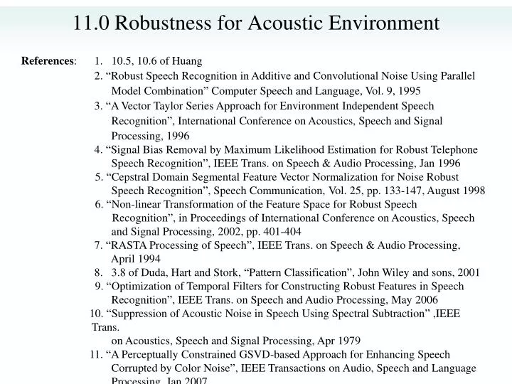
11.0 Robustness for Acoustic Environment References: 1. 10.5, 10.6 of Huang 2. “Robust Speech Recognition in Additive and Convolutional Noise Using Parallel Model Combination” Computer Speech and Language, Vol. 9, 1995 3. “A Vector Taylor Series Approach for Environment Independent Speech Recognition”, International Conference on Acoustics, Speech and Signal Processing, 1996 4. “Signal Bias Removal by Maximum Likelihood Estimation for Robust Telephone Speech Recognition”, IEEE Trans. on Speech & Audio Processing, Jan 1996 5. “Cepstral Domain Segmental Feature Vector Normalization for Noise Robust Speech Recognition”, Speech Communication, Vol. 25, pp. 133-147, August 1998 6. “Non-linear Transformation of the Feature Space for Robust Speech Recognition”, in Proceedings of International Conference on Acoustics, Speech and Signal Processing, 2002, pp. 401-404 7. “RASTA Processing of Speech”, IEEE Trans. on Speech & Audio Processing, April 1994 8. 3.8 of Duda, Hart and Stork, “Pattern Classification”, John Wiley and sons, 2001 9. “Optimization of Temporal Filters for Constructing Robust Features in Speech Recognition”, IEEE Trans. on Speech and Audio Processing, May 2006 10. “Suppression of Acoustic Noise in Speech Using Spectral Subtraction” ,IEEE Trans. on Acoustics, Speech and Signal Processing, Apr 1979 11. “A Perceptually Constrained GSVD-based Approach for Enhancing Speech Corrupted by Color Noise”, IEEE Transactions on Audio, Speech and Language Processing, Jan 2007
y[n] W=w1w2...wR x[n] Search Feature Extraction O =o1o2…oT O =o1o2…oT h[n] output sentences input signal original speech feature vectors acoustic reception microphone distortion phone/wireless channel n2(t) n1(t) Text Corpus Speech Corpus Acoustic Models Lexicon Language Model additive noise additive noise convolutional noise Acoustic Models x[n] Feature Extraction Model Training i = (Ai , Bi , i ) (training) Acoustic Models (recognition) Search and Recognition Feature Extraction O’ =o’1o’2…o’T y[n] ’i = (A’i , B’i , ’i ) Feature-based Approaches Model-based Approaches Speech Enhancement Mismatch in Statistical Speech Recognition • Mismatch between Training/Recognition Conditions • Mismatch in Acoustic Environment Environmental Robustness • additive/convolutional noise, etc. • Mismatch in Speaker Characteristics Speaker Adaptation • Mismatch in Other Acoustic Conditions • speaking mode:read/prepared/conversational/spontaneous speech, etc. • speaking rate, dialects/accents, emotional effects, etc. • Mismatch in Lexicon Lexicon Adaptation • out-of-vocabulary(OOV) words, pronunciation variation, etc. • Mismatch in Language Model Language Model Adaptation • different task domains give different N-gram parameters, etc. • Possible Approaches for Acoustic Environment Mismatch
Basic Idea primarily handling the additive noise the best recognition accuracy can be achieved if the models are trained with matched noisy speech, which is impossible a noise model is generated in real-time from the noise collected in the recognition environment during silence period combining the noise model and the clean-speech models in real-time to generate the noisy-speech models Basic Approaches performed on model parameters in cepstral domain noise and signal are additive in linear spectral domain rather than the cepstral domain, so transforming the parameters back to linear spectral domain for combination allowing both the means and variances of a model set to be modified Parameters used : the clean speech models a noise model Clean speech HMM Noisy speech HMM Cepstral domain C-1 C Noise HMM exp log Model combination Linear Spectral domain Model-based Approach Example 1― Parallel Model Combination (PMC)
Linear power spectral domain X()=S() +N() Xl=log(X), Sl=log(S)S=exp(Sl)Nl=log(N) N=exp(Nl) log exp Log spectral domain Xc=CXl, Sc=CSlSl=C-1ScNc=CNlNl=C-1Nc Nonlinear combination C C-1 Cepstral domain Model-based Approach Example 1 ― Parallel Model Combination (PMC) • The Effect of Additive Noise in the Three Different Domains and the Relationships
The Steps of Parallel Model Combination (Log-Normal Approximation) : based on various assumptions and approximations to simplify the mathematics and reduce the computation requirements Log-spectral domain Linear spectral domain Cepstral domain Noise HMM’s Clean speech HMM’s Noisy speech HMM’s Model-based Approach Example 1 ― Parallel Model Combination (PMC)
n 2 n n i, j: dimension index l l l Model-based Approach Example 2― Vector Taylor’s Series (VTS) • Basic Approach • Similar to PMC, the noisy-speech models are generated by combination of clean speech HMM’s and the noise HMM • Unlike PMC, this approach combines the model parameters directly in the log-spectral domain using Taylor’s Series approximation • Taylor’s Series Expansion for l-dim functions: • Given a nonlinear function z=g(x, y) • x, y, z are n-dim random vectors • assuming the mean of x, y, μx, μy and covariance of x, y, Σx, Σy are known • then the mean and covariance of z can be approximated by the Vector Taylor’s Series • Now Replacing z=g (x, y) by the Following Function • the solution can be obtained
Feature-based Approach Example 1— Cepstral Moment Normalization (CMS, CMVN) and Histogram Equalization (HEQ) • Cepstral Mean Subtraction(CMS) - Originally for Covolutional Noise • convolutional noise in time domain becomes additive in cepstral domain (MFCC) y[n] = x[n]h[n] y = x+h , x, y, h in cepstral domain • most convolutional noise changes only very slightly for some reasonable time interval x = yh if h can be estimated • Cepstral Mean Subtraction(CMS) • assuming E[x] = 0 , then E[y] = h , averaged over an utterance or a moving window, or a longer time interval xCMS= yE[y] • CMS features are immune to convolutional noise x[n] convolved with any h[n] gives the same xCMS • CMS doesn't change delta or delta-delta cepstral coefficients • Signal Bias Removal • estimating h by the maximum likelihood criteria h*= arg max Prob[Y = (y1y2…yT) | , h] , : HMM for the utterance Y • iteratively obtained via EM algorithm • CMS, Cepstral Mean and Variance Normalization (CMVN) and Histogram Equalization (HEQ) • CMS equally useful for additive noise • CMVN: variance normalized as well • HEQ: the whole distribution equalized • Successful and popularly used h xCMVN= xCMS/[Var(xCMS)]1/2 y=CDFy-1[CDFx(x)]
Temporal Filtering each component in the feature vector (MFCC coefficients) considered as a signal or “time trajectories” when the time index (frame number) progresses the frequency domain of this signal is called the “modulation frequency” performing filtering on these signals RASTA Processing : assuming the rate of change of nonlinguistic components in speech (e.g. additive and convolutional noise) often lies outside the typical rate of the change of the vocal tract shape designing filters to try to suppress the spectral components in these “time trajectories” that change more slowly or quickly than this typical rate of change of the vocal tract shape a specially designed temporal filter for such “time trajectories” MFCC Features B(z) yt B(z) B(z) Frame index feature vectors Modulation Frequency (Hz ) Feature-based Approach Example 2 ― RASTA ( Relative Spectral) Temporal Filtering New Features Frame index
PCA-derived temporal filtering temporal filtering is equivalent to the weighted sum of a sequence of a specific MFCC coefficient with length L slided along the frame index maximizing the variance of such a weighted sum is helpful in recognition the impulse response of Bk(z) can be the first eigenvector of the covariance matrix for zk ,for example Bk(z) is different for different k B1(z) B2(z) Original feature stream yt Bn(z) Frame index L zk(1) zk(2) zk(3) Features-based Approach Example 3 ― Data-driven Temporal Filtering (1)
Linear Discriminative Analysis (LDA) while PCA tries to find some “principal components” to maximize the variance of the data, the Linear Discriminative Analysis (LDA) tries to find the most “discriminative” dimensions of the data among classes Problem Definition wj, j and Uj are the weight (or number of samples), mean and covariance for the random vectors of class j, j=1……N,μis the total mean find W=[w1 w2 ……wk], a set of orthonormal basis such that tr(M): trace of a matrix M, the sum of eigenvalues, or the “total scattering” WTSB,WW: the matrix SB,W after projecting on the new dimensions Solution the columns of W are the eigenvectors of Sw-1SB with the largest eigenvalues Linear Discriminative Analysis (LDA)
LDA/MCE-derived Temporal Filtering For a specific timetrajectory k Frame index 1 2 3 4 5 Divided into classes LDA/MCE criteria zk(1) zk(2) zk(3) 3 LDA/MCE-derived filter 2 Class 1 zk (wk1 , wk2, wk3 )=wkT xk=wkTzk New time trajectoryof features Features-based Approach Example 3 ― Data-driven Temporal Filtering (2) • Filtered parameters are weighted sum of parameters along the time trajectory (or inner product)
Speech Enhancement producing a better signal by trying to remove the noise for listening purposes or recognition purposes Background Noise n[n] changes fast and unpredictably in time domain, but relatively slowly in frequency domain, N(w) y[n] = x[n] + n[n] Spectrum Subtraction |N(w)| estimated by averaging over M frames of locally detected silence parts, or up-dated by the latest detected silence frame |N(w)|i= β|N(w)|i-1+(1- β)|N(w)|i,n |N(w)|i: |N(w)| used at frame i |N(w)|i,n : latest detected at frame i signal amplitude estimation |X(w)|i = |Y(w)|i- |N(w)|i , if |Y(w)|i- |N(w)|i>α |Y(w)|i =α |Y(w)|i if |Y(w)|i- |N(w)|i≤α |Y(w)|i transformed back to x[n] using the original phase performed frame by frame useful for most cases, but may produce some “musical noise” as well many different improved versions ^ ^ Speech Enhancement Example 1 ― Spectral Subtraction (SS)
Signal Subspace Approach representing signal plus noise as a vector in a K-dimensional space signals are primarily spanned in a m-dimensional signal subspace the other K-m dimensions are primarily noise projecting the received noisy signal onto the signal subspace An Example Hankel-form matrix signal samples: y1y2y3…yk…yL…yM y1 y2 y3 y4… yk y2 y3 y4…… yk+1 Hy= y3 y4……….yk+2 . . . . . . . . . . . . yL yL+1 yM Generalized Singular Value Decomposition (GSVD) UTHyX = C =diag(c1, c2, …ck), c1≥c2≥… ≥ck VTHnX = S =diag(s1, s2, …sk), s1≤s2≤…≤sk subject to U, V, X : matrices composed by orthogonal vectors Which gives ci > si for 1 ≤ i ≤ m, signal subspace si > ci for m+1 ≤ i ≤ k, noise subspace Speech Enhancement Example 2 ― Signal Subspace Approach - Hy for noisy speech - Hn for noise frames
Audio Masking Thresholds without a masker, signal inaudible if below a “threshold in quite” low-level signal (maskee) can be made inaudible by a simultaneously occurring stronger signal (masker). masking threshold can be evaluated global masking thresholds obtainable from many maskers given a frame of speech signals make noise components below the masking thresholds Wiener Filtering estimating clean speech from noisy speech in the sense of minimum mean square error given statistical characteristics x(t) clean speech n(t) noise an example solution : assuming x(t), n(t) are independent Speech Enhancement Examples 3 and 4 ― Audio Masking Thresholds and Wiener Filtering y(t) E[(y(t)-x(t))2]=min