Download
1 / 5
50 likes | 160 Views
Mass Customization and the Learning Curve Appendix 7A. Mass customization is the new trend of making products partially mass produced, and partially customized.

E N D
Mass Customization and the Learning CurveAppendix 7A • Mass customization is the new trend of making products partially mass produced, and partially customized. • Land’s End sells mass produced clothing in catalogs and in stores such as Sears, but it also offers the service of stitching initials or names in shirts or duffle bags – this makes the product at the same time mass produced and customized. • Economies offered in the mass production of items helps to offset the expense of individually designed products. 2005 South-Western Publishing
Learning Curve Relationship • “Learning by doing" has wide application in production processes. • Workers and management become more efficient with experience. • The cost of production declines as the accumulated past production, Q = qt, increases, where qt is the amount produced in the tth period, and Q is the accumulated past production. • Airline manufacturing, ship building, and appliance manufacturing have demonstrated the learning curve effect.
Functionally, the learning curve relationship can be written C = a·Qb, where C is the input cost of the Qth unit: • Taking the (natural) logarithm of both sides, we get: log C = log a + b·log Q • The coefficient b tells us the extent of the learning curve effect. • If the b = 0, then costs are at a constant level. • If b > 0, then costs rise in output, which is exactly opposite of the learning curve effect. • If b < 0, then costs decline in output, as predicted by the learning curve effect.
Example • Cookie Baskets, Inc., is a local firm that assembles gift baskets. This is a one-owner, one-worker firm. Using data on time it takes to make the tenth, twentieth, and so forth baskets, the manager estimates the following regression. Ln T = .4 - .02 • Q R2 = .834 N = 30 (3.1) (2.6) where T is time it took to make a basket and Q is the accumulated number of baskets made, and the parentheses contain t-statistics. Q: Is this firm finding any benefits of Learning by Doing? A: Yes, the coefficient on Q is negative, so it takes less time to make baskets as the number of baskets made grows. The coefficient is statistically significant.
Percentage of Learning • The proportion by which costs are reduced through DOUBLING output is estimated as follows: L = (C2/C1)·100% • where C1 is the input or cost for the Q1 unit of output and C2 is the input or cost for the Q2 unit of output (and Q2 = 2•Q1). • If the percentage of learning, L = 82%, then input costs decline 18% as output doubles. • Thepercentage of learningis100% - L. • When L = 100%, there is no percentage of learning.