Download
1 / 50
510 likes | 659 Views
Scheduling Algorithms. Gursharan Singh Tatla professorgstatla@gmail.com. Scheduling Algorithms. CPU Scheduling algorithms deal with the problem of deciding which process in ready queue should be allocated to CPU. Following are the commonly used scheduling algorithms:. Scheduling Algorithms.

E N D
Scheduling Algorithms Gursharan Singh Tatla professorgstatla@gmail.com www.eazynotes.com
Scheduling Algorithms • CPU Scheduling algorithms deal with the problem of deciding which process in ready queue should be allocated to CPU. • Following are the commonly used scheduling algorithms: www.eazynotes.com
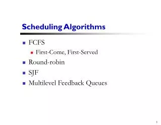
Scheduling Algorithms • First-Come-First-Served (FCFS) • Shortest Job First (SJF) • Priority Scheduling • Round-Robin Scheduling (RR) • Multi-Level Queue Scheduling (MLQ) • Multi-Level Feedback Queue Scheduling (MFQ) www.eazynotes.com
First-Come-First-Served Scheduling (FCFS) • In this scheduling, the process that requests the CPU first, is allocated the CPU first. • Thus, the name First-Come-First-Served. • The implementation of FCFS is easily managed with a FIFO queue. Ready Queue CPU D C B A Tail of Queue Head of Queue www.eazynotes.com
First-Come-First-Served Scheduling (FCFS) • When a process enters the ready queue, its PCB is linked to the tail of the queue. • When CPU is free, it is allocated to the process which is at the head of the queue. • FCFS scheduling algorithm is non-preemptive. • Once the CPU is allocated to a process, that process keeps the CPU until it releases the CPU, either by terminating or by I/O request. www.eazynotes.com
Example of FCFS Scheduling • Consider the following set of processes that arrive at time 0 with the length of the CPU burst time in milliseconds: www.eazynotes.com
P1 P2 P3 0 24 27 30 Example of FCFS Scheduling • Suppose that the processes arrive in the order: P1, P2, P3. • The Gantt Chart for the schedule is: • Waiting Time for P1 = 0 milliseconds • Waiting Time for P2 = 24 milliseconds • Waiting Time for P3 = 27 milliseconds www.eazynotes.com
Example of FCFS Scheduling • Average Waiting Time = (Total Waiting Time) / No. of Processes = (0 + 24 + 27) / 3 = 51 / 3 = 17 milliseconds www.eazynotes.com
P2 P3 P1 0 3 6 30 Example of FCFS Scheduling • Suppose that the processes arrive in the order: P2, P3, P1. • The Gantt chart for the schedule is: • Waiting Time for P2 = 0 milliseconds • Waiting Time for P3 = 3 milliseconds • Waiting Time for P1 = 6 milliseconds www.eazynotes.com
Example of FCFS Scheduling • Average Waiting Time = (Total Waiting Time) / No. of Processes = (0 + 3 + 6) / 3 = 9 / 3 = 3 milliseconds • Thus, the average waiting time depends on the order in which the processes arrive. www.eazynotes.com
Shortest Job First Scheduling (SJF) • In SJF, the process with the least estimated execution time is selected from the ready queue for execution. • It associates with each process, the length of its next CPU burst. • When the CPU is available, it is assigned to the process that has the smallest next CPU burst. • If two processes have the same length of next CPU burst, FCFS scheduling is used. • SJF algorithm can be preemptive or non-preemptive. www.eazynotes.com
Non-Preemptive SJF • In non-preemptive scheduling, CPU is assigned to the process with least CPU burst time. • The process keeps the CPU until it terminates. • Advantage: • It gives minimum average waiting time for a given set of processes. • Disadvantage: • It requires knowledge of how long a process will run and this information is usually not available. www.eazynotes.com
Preemptive SJF • In preemptive SJF, the process with the smallest estimated run-time is executed first. • Any time a new process enters into ready queue, the scheduler compares the expected run-time of this process with the currently running process. • If the new process’s time is less, then the currently running process is preempted and the CPU is allocated to the new process. www.eazynotes.com
Example of Non-Preemptive SJF • Consider the following set of processes that arrive at time 0 with the length of the CPU burst time in milliseconds: www.eazynotes.com
P1 P4 P3 P2 0 9 16 24 3 Example of Non-Preemptive SJF • The Gantt Chart for the schedule is: • Waiting Time for P4 = 0 milliseconds • Waiting Time for P1 = 3 milliseconds • Waiting Time for P3 = 9 milliseconds • Waiting Time for P2 = 16 milliseconds www.eazynotes.com
Example of Non-Preemptive SJF • Average Waiting Time = (Total Waiting Time) / No. of Processes = (0 + 3 + 9 + 16 ) / 4 = 28 / 4 = 7 milliseconds www.eazynotes.com
Example of Preemptive SJF • Consider the following set of processes. These processes arrived in the ready queue at the times given in the table: www.eazynotes.com
P1 P2 P4 P1 P3 5 26 0 1 10 17 Example of Preemptive SJF • The Gantt Chart for the schedule is: • Waiting Time for P1 = 10 – 1 – 0 = 9 • Waiting Time for P2 = 1 – 1 = 0 • Waiting Time for P3 = 17 – 2 = 15 • Waiting Time for P4 = 5 – 3 = 2 www.eazynotes.com
Example of Preemptive SJF • Average Waiting Time = (Total Waiting Time) / No. of Processes = (9 + 0 + 15 + 2) / 4 = 26 / 4 = 6.5 milliseconds www.eazynotes.com
Explanation of the Example • Process P1 is started at time 0, as it is the only process in the queue. • Process P2 arrives at the time 1 and its burst time is 4 milliseconds. • This burst time is less than the remaining time of process P1 (7 milliseconds). • So, process P1 is preempted and P2 is scheduled. www.eazynotes.com
Explanation of the Example • Process P3 arrives at time 2. Its burst time is 9 which is larger than remaining time of P2 (3 milliseconds). • So, P2 is not preempted. • Process P4 arrives at time 3. Its burst time is 5. Again it is larger than the remaining time of P2 (2 milliseconds). • So, P2 is not preempted. www.eazynotes.com
Explanation of the Example • After the termination of P2, the process with shortest next CPU burst i.e. P4 is scheduled. • After P4, processes P1 (7 milliseconds) and then P3 (9 milliseconds) are scheduled. www.eazynotes.com
Priority Scheduling • In priority scheduling, a priority is associated with all processes. • Processes are executed in sequence according to their priority. • CPU is allocated to the process with highest priority. • If priority of two or more processes are equal than FCFS is used to break the tie. www.eazynotes.com
Priority Scheduling • Priority scheduling can be preemptive or non-preemptive. • Preemptive Priority Scheduling: • In this, scheduler allocates the CPU to the new process if the priority of new process is higher tan the priority of the running process. • Non-Preemptive Priority Scheduling: • The running process is not interrupted even if the new process has a higher priority. • In this case, the new process will be placed at the head of the ready queue. www.eazynotes.com
Priority Scheduling • Problem: • In certain situations, a low priority process can be blocked infinitely if high priority processes arrive in the ready queue frequently. • This situation is known as Starvation. www.eazynotes.com
Priority Scheduling • Solution: • Aging is a technique which gradually increases the priority of processes that are victims of starvation. • For e.g.: Priority of process X is 10. • There are several processes with higher priority in the ready queue. • Processes with higher priority are inserted into ready queue frequently. • In this situation, process X will face starvation. www.eazynotes.com
Priority Scheduling (Cont.): • The operating system increases priority of a process by 1 in every 5 minutes. • Thus, the process X becomes a high priority process after some time. • And it is selected for execution by the scheduler. www.eazynotes.com
Example of Priority Scheduling • Consider the following set of processes that arrive at time 0 with the length of the CPU burst time in milliseconds. The priority of these processes is also given: www.eazynotes.com
Example of Priority Scheduling • The Gantt Chart for the schedule is: • Waiting Time for P2 = 0 • Waiting Time for P5 = 1 • Waiting Time for P1 = 6 • Waiting Time for P3 = 16 • Waiting Time for P4 = 18 0 1 6 16 18 19 www.eazynotes.com
Example of Priority Scheduling • Average Waiting Time = (Total Waiting Time) / No. of Processes = (0 + 1 + 6 + 16 + 18) / 5 = 41 / 5 = 8.2 milliseconds www.eazynotes.com
Another Example of Priority Scheduling • Processes P1, P2, P3 are the processes with their arrival time, burst time and priorities listed in table below: www.eazynotes.com
Another Example of Priority Scheduling • The Gantt Chart for the schedule is: • Waiting Time for P1 = 0 + (8 – 1) = 7 • Waiting Time for P2 = 1 + (4 – 2) = 3 • Waiting Time for P3 = 2 8 0 1 2 4 17 www.eazynotes.com
Another Example of Priority Scheduling • Average Waiting Time = (Total Waiting Time) / No. of Processes = (7 + 3 + 2) / 3 = 12 / 3 = 4 milliseconds www.eazynotes.com
Round Robin Scheduling (RR) • In Round Robin scheduling, processes are dispatched in FIFO but are given a small amount of CPU time. • This small amount of time is known as Time Quantum or Time Slice. • A time quantum is generally from 10 to 100 milliseconds. www.eazynotes.com
Round Robin Scheduling (RR) • If a process does not complete before its time slice expires, the CPU is preempted and is given to the next process in the ready queue. • The preempted process is then placed at the tail of the ready queue. • If a process is completed before its time slice expires, the process itself releases the CPU. • The scheduler then proceeds to the next process in the ready queue. www.eazynotes.com
Round Robin Scheduling (RR) • Round Robin scheduling is always preemptive as no process is allocated the CPU for more than one time quantum. • If a process’s CPU burst time exceeds one time quantum then that process is preempted and is put back at the tail of ready queue. • The performance of Round Robin scheduling depends on several factors: • Size of Time Quantum • Context Switching Overhead www.eazynotes.com
Example of Round Robin Scheduling • Consider the following set of processes that arrive at time 0 with the length of the CPU burst time in milliseconds: • Time quantum is of 2 milliseconds. www.eazynotes.com
Example of Round Robin Scheduling • The Gantt Chart for the schedule is: • Waiting Time for P1 = 0 + (6 – 2) + (10 – 8) + (13 – 12) = 4 + 2 + 1 = 7 • Waiting Time for P2 = 2 + (8 – 4) + (12 – 10) = 2 + 4 + 2 = 8 • Waiting Time for P3 = 4 0 2 4 6 8 10 12 13 15 17 www.eazynotes.com
Example of Round Robin Scheduling • Average Waiting Time = (Total Waiting Time) / No. of Processes = (7 + 8 + 4) / 3 = 19 / 3 = 6.33 milliseconds www.eazynotes.com
Multi-Level Queue Scheduling (MLQ) • Multi-Level Queue scheduling classifies the processes according to their types. • For e.g.: a MLQ makes common division between the interactive processes (foreground) and the batch processes (background). • These two processes have different response times, so they have different scheduling requirements. • Also, interactive processes have higher priority than the batch processes. www.eazynotes.com
Multi-Level Queue Scheduling (MLQ) • In this scheduling, ready queue is divided into various queues that are called subqueues. • The processes are assigned to subqueues, based on some properties like memory size, priority or process type. • Each subqueue has its own scheduling algorithm. • For e.g.: interactive processes may use round robin algorithm while batch processes may use FCFS. www.eazynotes.com
Multi-Level Queue Scheduling (MLQ) www.eazynotes.com
Multi-Level Feedback Queue Scheduling (MFQ) • Multi-Level Feedback Queue scheduling is an enhancement of MLQ. • In this scheme, processes can move between different queues. • The various processes are separated in different queues on the basis of their CPU burst times. • If a process consumes a lot of CPU time, it is placed into a lower priority queue. • If a process waits too long in a lower priority queue, it is moved into higher priority queue. • Such an aging prevents starvation. www.eazynotes.com
Multi-Level Feedback Queue Scheduling (MFQ) www.eazynotes.com
Multi-Level Feedback Queue Scheduling (MFQ) • The top priority queue is given smallest CPU time quantum. • If the quantum expires before the process terminates, it is then placed at the back of the next lower queue. • Again, if it does not complete, it is put to the last priority queue. • The processes in this queue runs on FCFS scheduling. • If a process becomes a victim of starvation, it is promoted to the next higher priority queue. www.eazynotes.com
Thank You Have a Nice Day www.eazynotes.com