Download
1 / 49
490 likes | 586 Views
Using optical experiments to quantitate intracellular calcium signals. On work in collaboration with: Luciana Bruno (UBA) Guillermo Solovey (UBA) Daniel Fraiman (U San Andres) Alejandra Ventura (Umich/UBA) Ian Parker (UC-Irvine) Sheila Dargan. Silvina Ponce Dawson

E N D
Using optical experiments to quantitate intracellular calcium signals. On work in collaboration with: Luciana Bruno (UBA) Guillermo Solovey (UBA) Daniel Fraiman (U San Andres) Alejandra Ventura (Umich/UBA) Ian Parker (UC-Irvine) Sheila Dargan Silvina Ponce Dawson Universidad de Buenos Aires Experiments @ UBA: work with Lorena Sigaut, Maria Laura Ponce, Lucia Halac, Estafania Piegari.
Calcium is a universal second messenger. It is involved in a large variety of processes, e.g.: Fertilization Cell death Neuronal communication, excitability and memory Muscle contraction and heart beat Intracellular calcium waves. Fontanilla and Nuccitelli Intercellular calcium waves Propagation of the leading edge of a Ca2+ wave in the rat retina. Video shown at normal speed. Width of image, 240 mm. Waves initiated with mechanical stimulus (10 msec, 15 -25 mm). Newman and Zahs, Science, 2758441997 Calcium signals travel as waves inside cells and between cells. Waves involve calcium release from internal stores such as the endoplasmic reticulum.
Optical methods provide a relatively non-invasive means by which calcium signals can be studied. This is the approach followed by I. Parker (UC-Irvine) who studies calcium signals in intact cellswhere calcium is released from the ER through IP3R/Ca2+ channels.
Optical experiments have led to the conclusion that IP3 receptors are organized in clusters. Thus, a variety of signals can be evoked depending on the amount of IP3: Figs. by I. Parker’s group.
One of the quantities we want to infer from optical experiments is the amplitude and time course of the calcium current that underlies each signal. This is not easy because several processes affect the Ca2+ dynamics once it is released into the cytosol. When calcium is released from the ER, it diffuses and interacts with other species (buffers, pumps, etc) that compete with the dye for calcium. Fig. from Martin D Bootman and Peter Lipp, Calcium Signalling and Regulation of Cell Function Not only the [Ca2+] but also Ca2+ diffusion is affected by the presence of buffers one of which is the fluorescent indicator that is used to visualize the signals.
The presence of different types of buffers can completely alter the observed dynamics, what about the dye? Experiments I Parker’s lab Different methods had been proposed in the literature to go from the image to the Ca2+ currents. They all involved having a very detailed model of the cytosolic Ca2+ dynamics. In 2005 we proposed a method that was based on ideas of dynamical systems theory and which does not need a detailed working model of the intracellular calcium dynamics, but infers some of its properties from the images themselves. It is useful in the case of localized signals (with identifiable regions where there is release and others where there is not).
Suppose we have an experiment in which only one variable can be measured as a function of time, i.e., we have a (scalar) time series, u(t). If the time series is sufficiently long, then by observing the past evolution it is possible to “predict” the future. Using u(t) and its derivatives (equivalently, knowing u at the present time and at previous times) we can construct a dynamical system that reproduces the observed time series (that predicts what is going to happen next). All the relevant information is contained in the time series!
The first steps of our method (Ventura et al, Biophys J, 2005) The image occurs because calcium binds to the dye, F. F: fluo4 The fluorescence, f, and [CaF] are related by: [F]T is known fmin and fmax can be measured. [CaF] evolves according to: Assuming spherical symmetry, we can compute time and space derivatives of [CaF](r,t) and obtain [Ca2+](r,t)…
We have a spatio-temporal series of the calcium concentration. Analyzing its behavior in the regions where there is no calcium release, we extract information on the processes that remove calcium. Using this information in the regions where there is release, we infer the underlying current. Here I will show the results of applying this “model independent” method to determine the calcium current that underlies calcium puffs in Xenopus laevis oocytes.
Application to 2 sets of experiments done with 2 dyes: Fluo4 and Oregon green. Main results with Fluo 4. EGTA was also injected in the cells. Averaged and raw puffs give more or less the same distributions. Data obtained with different flash durations are indistinguishable. We work with averaged puffs pooling all data together and obtain the properties of the calcium current that underlies each observation (A) Various puffs (B) One of the puffs in A (marked by black box). (C) Similar to B, but averaged (D) Averaging procedure. Five raw puffs and averaged one (lowest image) (E and F) Temporal and spatial profiles of the puff in B (H) Spatial profile of the source at the time of maximal signal. Circles: experimental data; solid line: Gaussian fit. (I) Solid line: current time Bruno et al, Cell Calcium (2010)
Various distributions Notice lr pretty uniform (different from lf) (A and B) Normalized distributions of peak fluorescence amplitude of averaged puffs for Fluo-4 (n = 117) and Oregon green (n = 406) experiments. (C). Distribution of rise times tf for Fluo-4 experiments. (D and E) Distributions of Ca2+ flux durations tr for Fluo-4 and Oregon green experiments, respectively. (F–H) Similar to C–E, but for puff (lf) and Ca2+ source (lr) sizes.
Current distribution fI(I) (A) Maximum current value distribution from 105 averaged puffs of Fluo-4 experiments. (B) Dependence of puff amplitude on the maximum current during release (Fluo-4 experiments). Black and open circles correspond to simulations C. Similar to A but for 364 puffs of Oregon green experiments. fI(I)I= number of puffs with current between I and I+I First attempt to go from fI(I) to distribution of “puff sizes” • # of open channels, No, proportional to # of IP3R’s with IP3 bound, Np, given by a Poisson distribution (neglect cluster to cluster variability) • I=Io No, solid,and , dashed • Io and <No> from fitting Not very good (inter-cluster variability important)
First summary We used a previously developed algorithm to analyze the properties of Ca2+ release during puffs and found the following: The calcium release duration varies between 6 and 35 ms and is peaked around 18ms. Calcium release comes from a region of width ~ 460 nm, which does not vary much from puff to puff. This led us to the conclusion that different clusters mainly differ in their IP3R densities. The calcium currents range between 0.12 and 0.95pA, independently of the [IP3] value. Cluster to cluster variability plays an important role in shaping the distributions of puff sizes and calcium currents. More on how to use modeling to extract info on intra-cluster organization from these results in the informal talk
But… How reliable are these results? Let us remember the first steps of the method to infer the calcium current: We went from F to [CaF] where [F]T is known fmin and fmax can be measured. Then computed space and time derivatives of [CaF] and from: obtained [Ca2+] as function of space and time.
For which we need to know DF, k+, k- The vendor of the dye provides KD=k-/k+, but what about the rest? Furthermore, our method also needs to know the free diffusion coefficient of calcium (more on this later). How sensitive are the results that we obtain to variations in these parameters? We applied our method to a series of numerically generated images. We knew all the parameter values and the calcium current for these images. We applied the method using other parameter values and computed the relative error of the determined current.
Parameters used to generate the images and ranges of values over which we chose the ones we used to determine the current. The results are mainly sensitive to errors in the diffusion coefficients.
How fast does calcium diffuse in the cytosol? Mechanisms that modulate the distribution of intracellular calcium. From MD Bootman and P Lipp, Calcium Signalling and Regulation of Cell Function Fig. by Ian Parker’s lab Calcium does not diffuse freely inside the cytosol Hard to answer because: The fastest trapping mechanism is buffering. Buffers diffuse more slowly than calcium ions, thus, they slow down the transport of calcium. Buffers modulate calcium signals changing them dramatically
Calcium transport inside the cytosol can be described in terms of an effective diffusion coefficient (which depends on calcium). Simplest case: A = Ca2+
The dependence of D with [Ca2+] can be obtained, e.g., within the rapid buffering approximation Example: calcium in presence of one buffer It assumes that the reaction with the buffers occurs much faster than all other processes, including diffusion. + q ¶ D D w = Ñ + 2 Ca B ( w f ) with ¶ + q t 1 It can be approximated by (Wagner and Keizer, 1994; Sneyd et al, 1998):
It is hard to determine the free diffusion coefficient of any substance in an environment in which it interacts with other species (like it occurs with calcium in the cytosol). This occurs with a technique that is used very widely to determine the diffusion of proteins: FRAP. Experiments usually provide information on the effective diffusion coefficient in those cases.
In the case of calcium, its effective diffusion coefficient was estimated using radioactive Ca2+. Radioactive Ca2+ is added to a cytosolic extract and the radioactivity distribution is measured at various t’s. It’s fitted with a Gaussian and D is extracted. In some cases, non radioactive Ca2+ is added previously. Figures from Allbritton et al, Science’92. The studies we presented in PNAS (2006) 103: 5338-5342 show that there is more than one effective diffusion coefficient and that Dca could have been underestimated in the radioactive calcium experiments (to paper)
It is of interest to determine the calcium transport properties in the cell by some other means. We need to know its free diffusion coefficient and how much calcium is buffered (the buffering capacity of the cell). One method to study that: Fluorescent correlation spectroscopy FCS measures the correlation between fluorescence fluctuations within a detection volume of the order of 1 fl. Example with one fluorescent purely diffusing species: Compute autocorrelation of fluorescence:
For one purely diffusing species the correlation is given by: Fitting the experimental G(t) with this formula we obtain G0 and D. wxy is obtained from a calibration with a substance for which D is known. Thus, D can be determined from the experiment. Example (L. Sigaut, M. L. Ponce in confocal microscope): 50 nM TMR-Dex†† in water. Black: experimental data, red: fitting
FCS can also be used to determine effective diffusion coefficients of fluorescent particles that diffuse and react (formulas are more complicated) Fluorescent particles that diffuse and react with traps. Analytic approximation, up to 2nd order in wavenumber (long time limit, valid for reaction times shorter than diffusion times) with L. Sigaut 2nd component: 1st component: free trap diffusion coefficient Effective coefficient obtained is Du (FRAP gives Dt)
Ca2+ free non fluorescent * fluo 4 free non fluorescent Ca2+ bound fluo 4 fluorescent * * * * * * * * * * * * * * * * * * * * * * * * * FCS can also be used to determine effective diffusion coefficients of particles that fluoresce upon binding to another one (e.g., calcium and dye).
FCS. Formulas for calcium diffusing and reacting with a dye that fluoresces upon calcium binding Fluo4 free diffusion D1 effective diffusion coefficient D2 effective diffusion coefficient Where:
First observation: Formula depends on two effective diffusion coefficients (+ dye diffusion coefficient). How the two effective diffusion coefficients depend on the free dye concentration
Second Observation: The relative weight of the last two terms can be changed by changing the total calcium or dye concentrations. Thus: we can expect to get D1 and D2 from experiments done for different total concentrations of calcium or dye. What we did: Experiments in solution with constant dye concentration (F4tot) and different Ca2+ concentrations. Dye: Fluo 4 dextran. ( Molecular Probes- Invitrogen). Dissociation constants provided by vendor. In these experiments there is an extra calcium buffer (EGTA). Therefore, the “free” calcium diffusion coefficient that we may get from D2 and D1 is an effective calcium/EGTA diffusion coefficient.
Experiments in solution F4tot constant Point FCS, 10s/pixel. Solutions with different [Ca2+]. Turned out to be that the second component dominated the correlation function. We could fit the correlations for different F4tot’s using only the second component and the values we obtained were reasonable. Keeping only the second component we have:
Experiments in solution DCa= ( 334 +/- 262 ) um2/s DF4= ( 93 +/- 18 ) um2/s Fitting D2 Between parentheses expected values
Experiments in solution Kd = ( 781 +/- 257 ) nM F4tot = ( 720 +/- 6) nM Fitting Go Between parentheses expected values
Experiments in oocytes We started to do point FCS experiments in oocytes We did experiments using TMR to estimate dye free diffusion coefficient Experiments done with Fluo 4 at basal conditions are very noisy and we only found, so far, the first component (which agrees with the obtained free dye diffusion coefficient). In this case the condition is different than in solution, because the calcium diffusion coefficient that we are trying to estimate (an effective coefficient due to the interaction with endogenous buffers) is smaller than that of the dye. We are planning to repeat the experiments changing the free calcium concentration (interfering with SERCA, shining UV light on a pigment granule…)
Second summary We performed a series of point FCS experiments in solutions with different total calcium concentratons and a fixed value of the total dye concentration. This resulted in data sets with different free dye concentrations. We could fit the correlation functions using only the term that depended on one of the effective diffusion coefficients (D2). The fitting gave correct values for the Ca2+ effective diffusion, the calcium/dye dissociation constant and the total dye concentration. This shows the feasibility of the method and the accuracy of (part) of the analytic expression that we obtained for the correlation functions. Next step: do this in intact cells to extract information on calcium transport properties and buffering capacity. Preliminary results in basal conditions: too noisy (always get dye coefficient).
Final summary Calcium ions participate of a variety of biological processes. Optical experiments provide a relatively non-invasive means by which calcium signals can be studied. A combination of modeling and experiments is necessary to obtain a comprehensive description. Model building and data analyses require reliable values of the various biophysical parameters involved. We have recently started an experimental effort to determine these parameters in situ and in vivo and to obtain calcium signals ourselves. Results still preliminary Thank you!
Aims: • To insure exact comparability across countries—one report at the end of the process • To show whether women physicists’ experiences are different from men’s (Men must also reply to the questionnaire in order to answer this) • To provide survey in languages other than English Please fill in at: http://www.aipsurveys.org/global/
Let us go back now to the results we obtained from the analysis of calcium puffs and try to infer other properties Current distribution fI(I) fI(I)I= number of puffs with current between I and I+I Can we infer how many channels opened during each puff? If all IP3R’s opened at the same time and current through each of them was the same, Io: No=number of open IP3R’s=I/Io fI(I)I= number of events with No between I/Io and (I+I)/Io We would get probability of having puffs with No open IP3R’s but….
Going from fI(I) to distribution of “puff sizes” • Sources of variability of puff size: • events come from different clusters (different # of IP3R’s) • different # of IP3R’s with IP3 bound before each puff • First approach: • # of open channels, No, proportional to # of IP3R’s with IP3 bound, Np, given by a Poisson distribution (neglect 1st source of variability) • I=Io Noand From the fitting, determine unknown parameters Io, m Model I: one Poisson and =1 I=IoNp =1 (linear), =2 (Thul & Falcke) =1, Io=0.086pA, m=4 (solid lines) and =2, Io=0.45pA and m=0.72 (dashed curves).
The distribution seems to be bimodal: we try a superposition of Poisson distributions, (rationale: there are clusters with different numbers of IP3R’s) Best fit: superposition of two Poisson distributions plus nonlinear relationship between I and Np. Model II Io1N pt = I o2N pt1/2=I* 1= 1, 2= 2, I*=0.38pA , Io1 = 0.017 pA, m1=15, Io2 = 0.08pA, m2 = 33, 1= 0.7199 and 2= 0.27
Is this description better just because it has more adjustable parameters or does it really represent what is going on? Checking the plausibility of such a model with numerical simulations. First set of simulations: simple description of Ca2+ entry that does not include an IP3R kinetic model We solve the set of coupled reaction-diffusion equations that describe the dynamics of Ca2+ in the presence of one dye, EGTA and an immobile endogenous buffer, assuming the following geometry: Fixed spatial extent of the cluster, different number of open channels, different single channel current (to compare model with one and two Poissons).
Simple description of Ca2+ entry: We take a 500nmx500nm square and consider a (square) grid inside with nodes that are 20nm apart from one another For each simulation we pick a value of Np (# of IP3R’s with IP3 bound=# of open IP3R’s) from a Poisson distribution (as in model I) or the superposition of 2 Poisson distributions (as in model II) and choose Np nodes of the square grid at random (with uniform probability). We assume that all channels open and close simultaneously and remain open for 10ms. In the case of model I, we assume that the current Io flows through each of them. In the case of model II, we assume that the channel through each open IP3R, Is, depends on Np so that IsNp=I and Io1 = 0.017 pA Io1N pt = I o2N pt1/2=I* = 0.38pA
With the simulations we obtain the distribution of Ca2+-bound dye which we relate to the distribution of fluorescence by: (“blurring” the distribution first) Both models reproduce the amplitude to current relationship correctly (filled circles: Model I, open circles: Model II)
Simulations of trigger and puffs to check their ability to reproduce the puff to trigger amplitude distribution reported in Rose et al, 2006. In this case 3 IP3R’s open first and the rest open 10ms later: A. Three examples of the spatial distribution of IP3R’s (Np=5; Np=30; Np=55). B. Deterministic simulation of four puffs originated after a trigger event. For the first 12 ms only one channel is open. All other channels then open for 18 ms. Black traces are Np=5 and dotted traces Np=15. The two upper traces correspond to the linear model and the lower ones to the “best” model. C. Distribution of puff to trigger amplitude ratio derived from paired measurements as described in Rose et al (25) (vertical bars). Solid line with white dots indicate the expected ratio for the linear model and with filled circles the one for the “best” model.
The simulations favor Model II over Model I Current distribution functions for Fluo-4 (A and B) and Oregon green (D and E) experiments. Bars: experimental data. Lines: Theoretical expressions. (A) Poisson distribution and I~No with α = 1, Io = 0.086 pA, m = 4 (solid line) and with α = 2, Io = 0.45 pA and m = 0.72 (dashed curve). (B) Superposition of 2 Poissons and I vs No relationship as in C. (D, E, F): Similar to (A,B,C) but for Oregon green experiments. • Possible conclusions and/or interpretation: • Cluster to cluster variability plays an important role in shaping distribution of puff sizes. • Nonlinearity of I(Np) due to luminal Ca2+ depletion as more channels become open • Channel current of one open channel: 0.017pA
Then, we wanted to interpret other observations and extract other information on the behavior of single IP3R’s. Notice tr pretty independent from I Dependence of Ca2+ flux duration (tr) and of Ca2+ source size (lr) on the maximum current, Imax for Fluo-4 (A and B) and Oregon green (C and D) experiments. Standard deviations and bin sizes of current around mean values are represented with error bars. Is the observed independence of tr w.r.t. I a reflection of a similar behavior at the single channel level (mean open time independent of [Ca2+])? We need to include single channel kinetics in the model to answer this.
Remember model: Now: Ij =Is Xj, where Xj switches between 1 and 0 depending on the IP3R state which changes stochastically according to the IP3R kinetic model To answer the question we use two very simple kinetic models: We are not including IP3 binding and unbinding (we assume the number of IP3R’s with IP3 bound, Np, is fixed during each puff). Surprise: we could reproduce observations with a single channel current that was independent of the number of open channels and that was larger than the one estimated from the previous analysis!
Simulations including stochastic switchings of IP3R. Single channel current= 0.1pA always! Time evolution of the current (I) released through a cluster of Np=15 available IP3R’s (A) and of the resulting fluorescence signal, FR, (B) obtained with the stochastic simulations. Solid lines: model Cd gray lines: model Ci. Puff rising time (tf) and amplitude (A) illustrated in Fig. 2B. C-D: Same as A-B but for a cluster of Np=33 channels. Puff duration and maximum (smoothed) current released as functions of amplitude.
Main difference between previous simulations and these ones: IP3R’s do not open and close simultaneously now. Compute average released current to compare with previous simulations (which correspond to a “mean field” model): A Mean and standard deviation (bars) of puff amplitude as function of the number of available channels, Np, (mean with dots) and as a function of the maximum number of simultaneously open channels, n, (mean with solid circles) for stochastically simulated puffs model Cd. B: Average Ca2+ current released during a stochastically simulated puff as a function of the number of available channels. The solid line corresponds to the fitting I=Io1Np (Np≤22) and I=Io2Np½ (Np>22) which gives Io1=0.019pA and Io2=0.105pA. Io1should not be taken as the actual single IP3R current but as an effective value that follows from the assumption that all channels open and close simultaneously. Average current increases nonlinearly with Np and single channel current is similar to the one obtained with (mean field) Model II !!
About the question that motivated our study Stochastic puff model. (A) Puff duration (tf) as a function of puff amplitude for experimental observations in X. laevis oocytes (open circles) and stochastically simulated puffs obtained using model Cd (black squares and error bars correspond to mean values and standard deviations, respectively). (B) Duration of the Ca2+ release as a function of the maximum Ca2+ current for stochastically simulated puffs obtained using model Cd (black circles) and Ci (open circles). (C) Maximum released current (open circles) and averaged current (mean with black dots and standard deviation with vertical lines) released during the events as function of the number of channels in the cluster, Np, obtained with simulations that use the Cd kinetic model.
Analysis and models of Ca2+ puffs and clusters We used a previously developed algorithm to analyze the properties of Ca2+ release during puffs. We found that thisrelease comes from a region of width ~ 460 nm, which does not vary much from puff to puff. The estimated duration is peaked around 18ms and the underlying Ca2+ currents range between 0.12 and 0.95pA, independently of the [IP3] value. We found that the mean field model that best fits the observations is one in which there are at least two populations of clusters characterized by different mean numbers of channels and where the current scales nonlinearly with the number of open channels. Using simulations that include a description of the stochastic switchings between channel states (as opposed to mean field models in which all channels open and close simultaneously) we found that the nonlinearity and small single channel current of the “best” mean field model is a consequence of the averaging procedure implicit in this type of models. Even though mean field models cannot provide accurate information on single channel properties, they are still useful as building blocks of more global signals such as waves.