Download
1 / 21
210 likes | 407 Views
FAF2 Data Disaggregation Methodology and Results. presented to Model Task Force presented by Vidya Mysore, Florida DOT Krishnan Viswanathan, Cambridge Systematics, Inc. November 28, 2007. Presentation Overview. Background Florida FAF 2 data FAF 2 Disaggregation method

E N D
FAF2 Data DisaggregationMethodology and Results presented to Model Task Force presented by Vidya Mysore, Florida DOT Krishnan Viswanathan, Cambridge Systematics, Inc. November 28, 2007
Presentation Overview • Background • Florida FAF2 data • FAF2 Disaggregation method • Illustrative Example • Comparison with TRANSEARCH • Future Year Projections
Background • Growth in Florida • Increasing freight transportation • Capacity Constraints • FAF2 as potential data source • Audience of modelers and planners
Florida FAF2 Data • Forecasts based on overall economic changes • Mode shares are assumed same in future • 98 percent increase in commodity flows from 2002 to 2035 • Truck increase is 108 percent • Domestic Water will decline by 51 percent
FAF2 Disaggregation Method • Data Sources • FAF2 • County Business Pattern (CBP) • Public Use Microdata Samples (PUMS) • Census 2000 • Three digit NAICS employment at county level • CBP most complete at MSA • Therefore use PUMS for employment allocation • Census 2000 for government and self-employed
SCTG Table NAICS Table CBP Data Census 2000 and QCEW Data SCTG 2 to NAICS 3 Equivalency Table NAICS 3 Employment Table Mode Split to Truck (kTon) 2002 Economic Census Data Rail (kTon) Disaggregated to 2002 FAF2 Database County Level FAF2 Database by Value DOMESTIC (kTon) Water (kTon) SCTG 2 to NAICS 3 Equivalency Table BORDER (kTon) SEA (kTon) SCTG 2 to NAICS 3 Equivalency Table County Level FAF2 Database by Commodity 2002 FAF2 Database NAICS 3 Employment Table FAF2 Disaggregation Method
Mode Split to Truck (kTon) Rail (kTon) Water (kTon) FAF2 Disaggregation Method SCTG 2 to NAICS 3 Equivalency Table County Level FAF2 Database by Commodity 2002 FAF2 Database NAICS 3 Employment Table County Level FAF2 Database by Commodity TAZ Level FAF2 Database by FL Statewide Model Commodity Groupings 2005 InfoUSA Data
FAF2 Disaggregation Method • Develop relationships between commodity and employment and population data • Rationale is commodities end up in Zones that produce or consume them • Use relationships to develop factors for each commodity for freight flow disaggregation • Apply share of county tonnage to FAF2 regional tonnage to obtain disaggregated FAF2 O-D database
Illustrative Example Florida Statewide Freight Model
Illustrative Example • Paper (SCTG 27, 28) • Pulp, Newsprint, Paper, and Paperboard • Paper or Paperboard Articles • Production Equation • 0.362 (21.53) x Paper Manufacturing (NAICS 322) • R2 = 0.80 • Attraction Equation • 0.064 (4.56) x Paper Manufacturing (NAICS 322) + 0.043 (4.59) x Printing and Related (NAICS 323) • R2 = 0.76
Illustrative Example • Estimate the annual tonnage of paperproduced Pc(i) or attracted Ac(j) for each County • Aggregate the county productions Pc(i) and attractions Ac(j) to their associated Florida FAF2 regions to create PFAF2(i) and AFAF2(j) • Expand the FAF2 Regions matrix, FAF2(k,l), to Florida counties matrix, County (i,j)
Illustrative Example • If origin i and destination j are in Florida then County(i,j)=[FAF2(k,l)*Pc(i)/PFAF2(i)* Ac(j)/ AFAF2(j)] • If origin i is in Florida and destination l, is outside Florida then County(i,l)=[ FAF2(k,l)*Pc(i)/PFAF2(i)] • If origin k is outside Florida and destination j is in Florida then County(k,j)=[ FAF2(k,l)*Ac(j)/AFAF2(j)]
Comparison with TRANSEARCH • TRANSEARCH STCC 26 (Pulp, Paper, or Allied Products) • TRANSEARCH is unlinked trips and FAF2 is linked trips
Future Year Projections • Establish national control totals by commodity • Apply specific shipment growth by market and commodity • Apply specific purchasing and consumption growth by market and commodity
Future Year Projections • Summarize and compare results with national control totals • Adjust resulting freight flows so that volumes correspond with national level as follows: • For each market & commodity, adjust so shipments match purchases • For each commodity, adjust so that national control totals are satisfied
Future Year Projections • Use same methodology for Florida using CBP and Woodes & Poole (WP) data • WP data available at county level • Since we are focused on only tonnage, the data available to use can be used in a similar manner
Discussion http://farm2.static.flickr.com/1191/875522713_c71061093b.jpg?v=0