Download
1 / 100
1k likes | 1.16k Views
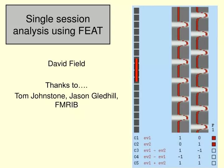
Single session analysis using FEAT. David Field Thanks to…. Tom Johnstone, Jason Gledhill, FMRIB. Single “session” or “first level” FMRI analysis. In FMRI you begin with 1000’s of time courses, one for each voxel location Lots of “preprocessing” is applied to maximise the quality of the data

E N D
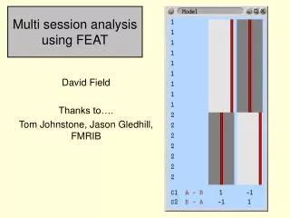
Single session analysis using FEAT David Field Thanks to…. Tom Johnstone, Jason Gledhill, FMRIB
Single “session” or “first level” FMRI analysis • In FMRI you begin with 1000’s of time courses, one for each voxel location • Lots of “preprocessing” is applied to maximise the quality of the data • Then, each voxel time course is modelled independently • the model is a set of regressors (EV’s) that vary over time • the same model is applied to every voxel time course • if (part of) the model fits the voxel time course well the voxel is said to be “active” 241 256 250 234 242 260 254
Plan for today • Detailed look at the process of modelling a single voxel time course • The input is a voxel time course of image intensity values and the design matrix, which is made up of multiple EV’s • The GLM is used to find the linear combination of EV’s that explains the most variance in the voxel time course • The output is a PE for each EV in the design matrix • Preprocessing of voxel time courses • this topic probably only makes much sense if you understand 1) above, which is why I am breaking with tradition and covering this topic second rather than first • Implementing a single session analysis in FSL using FEAT (workshop) • Note: There is no formal meeting in week 3 of the course, but the room will be open for you to complete worksheets from today and last week • at least one experienced FSL user will be here to help
The BET brain extraction option refers to the 4D functional series • This will not run BET on the structural • Normally turn this on • Brain extraction for the structural image that will be used as the target for registration has to be performed by you, before you use FEAT to set up the processing pipeline
On the Misc tab you can toggle balloon help • Balloon help will tell you what most of the options mean if you hover the mouse over a button or tickbox • But it gets annoying after a while • If progress watcher is selected then FEAT opens a web browser that shows regular updates of the stage your analysis has reached
Motion Correction: MCFLIRT • Aims to make sure that there is a consistent mapping between voxel X,Y,Z position and actual anatomical locations • Each image in the 4D series is registered using a 6 DOF rigid body spatial transform to the reference image (by default, the series mid point) • This means every image apart from the reference image is moved slightly • MCFLIRT plots the movements that were made as output
MCFLIRT output Head rotation Head translation Total displacement
The total displacement plot displacement is calculated relative to the volume in the middle of the time series Relative displacement is head position at each time point relative to the previous time point. Absolute displacement is relative to the reference image.
The total displacement plot Why should you be particularly concerned about high values in the relative motion plot? The first thing to do is look at the range of values plotted on the y axis, because MCFLIRT auto-scales the y axis to the data range
Slice timing correction Each slice in a functional image is acquired separately. Acquisition is normally interleaved, which prevents blending of signal from adjacent slices Assuming a TR of 3 seconds and, what is the time difference between the acquisition of adjacent slices? A single functional brain area may span two or more slices
Why are the different slice timings a problem? • The same temporal model (design matrix) is fitted to every voxel time course • therefore, the model assumes that all the voxel values in a single functional volume were measured simultaneously • Given that they are not measured simultaneously, what are the implications? • Consider two voxels from adjacent slices • both voxels are from the same functional brain area • this time the TR is 1.5, but the slice order differed from the standard interleaved procedure, so there is a 1 sec time gap between acquisition of two voxels in the adjacent slices that cover the functional brain area
Blue line = real HRF in response to a brief event at time 0 Blue squares: intensity values at a voxel first sampled at 0.5 sec, then every 1.5 sec thereafter (TR = 1.5) Red circles: intensity values at a voxel from an adjacent slice first sampled at 1.5 sec, then every 1.5 sec thereafter (TR = 1.5)
These are the two voxel time courses that are submitted to the model
The model time course is yoked to the mid point of the volume acquisition (TR), so there will be a better fit for voxels in slices acquired at or near that time. These are the two voxel time courses that are submitted to the model
Slice timing solutions • Any ideas based on what was covered earlier? • Including temporal derivatives of the main regressors in the model allows the model to be shifted in time to fit voxels in slices acquired far away from the mid point of the TR • But, • this makes it difficult to interpret the PE’s for the derivatives: do they represent slice timing, or do they represent variations in the underlying HRF? • and, you end up having to use F contrasts instead of t contrasts (see later for why this is to be avoided if possible)
Slice timing solutions • Any ideas based on what was covered earlier? • Use a block design with blocks long enough that the BOLD response is summated over a long time period • But, • Not all experimental stimuli / tasks can be presented in a block design • So, • another option is to shift the data from different slices in time by small amounts so that it is as if all slices were acquired at once • this is what the preprocessing option in FEAT does
Shifting the data in time - caveats • But if the TR is 3 seconds, and you need to move the data for a given slice by, e.g., 1 sec, you don’t have a real data point to use • get round this by interpolating the missing time points to allow whole voxel time courses to be shifted in time so effectively they were all sampled at once at the middle of the TR • But… • Interpolation works OK for short TR, but it does not work well for long TR (> 3 sec?) • So this solution only works well when slice timing issues are relatively minor • There is a debate about whether to do slice timing correction before or after motion correction • FSL does motion correction first • some people advise against any slice timing correction • Generally, if you have an event related design then use it, but make sure you check carefully with the scanner technician what order your slices were acquired in!
Temporal filtering • Filtering in time and/or space is a long-established method in any signal detection process to help "clean up" your signal • The idea is if your signal and noise are present at separable frequencies in the data, you can attenuate the noise frequencies and thus increase your signal to noise ratio
Very low frequency component, suggests that high pass filter also needed
Setting the high pass filter for FMRI • The rule recommended by FSL is that the lowest setting for the high pass filter should be equal to the duration of a single cycle of the design • In an ABCABCABC block design, it will be equal to ABC • If you set a shorter duration than this you will remove signal that is associated with the experiment • If you set a higher duration than this then any unsystematic variation (noise) in the data with a periodic structure lower in frequency than the experimental cycle time will remain in voxel time courses • In complicated event related designs lacking a strongly periodic structure there is a subjective element to the setting of the high pass filter
Setting the high pass filter for FMRI • Do not use experimental designs with many conditions where the duration of a single experimental cycle is very long • e.g. ABCDEABCDE, where ABCDE = 300 seconds • setting the high pass to 300 sec will allow a lot of the low frequency FMRI noise to pass through to the modelling stage • Furthermore, the noise can easily become correlated with the experimental time course because you are using an experimental time course that has a similar frequency to that of FMRI noise • In any signal detection experiment, not just FMRI, you need to ensure that the signal of interest and noise are present at different temporal frequencies
Low pass filter? • As well as removing oscillations with a longer cycle time than the experiment, you can also elect to remove oscillations with a higher cycle time than the experiment • high frequency noise • In theory this should enhance signal and reduce noise, and it was practiced in the early days of FMRI • However, it has now been demonstrated that because FMRI noise has temporal structure (i.e. it is not white noise), the low pass filter can actually enhance noise relative to signal • The temporal structure in the noise is called “temporal autocorrelation” and is dealt with in FSL using FILM prewhitening instead of low pass filtering • in another break with the traditional structure of FMRI courses temporal autocorrelation and spatial smoothing will be covered after t and F contrasts
After preprocessing and model fitting • You can now begin to answer the questions you set out to answer….
Which voxels “activated” in each experimental condition? • In the auditory / visual stimulus experiment, how do you decide if a voxel was more “activated” during the visual stimulus than the baseline? • If the visual condition PE is > 0 then the voxel is active • but > 0 has to take into account the noise in the data • We need to be confident that if you repeated the experiment many times the PE would nearly always be > 0 • How can you take the noise into account and quantify confidence that PE > 0? • PE / residual variation in the voxel time course • this is a t statistic, which can be converted to a p value by taking into account the degrees of freedom • The p value is the probability of a PE as large or larger than the observed PE if the true value of the PE was 0 (null hypothesis) and the only variation present in the data was random variation • FSL converts t statistics to z scores, simplifying interpretation because z can be converted to p without using deg of freedom
Why include “effects of no interest” in the model? • Also called “nuisance regressors” • Imagine an experiment about visual processing of faces versus other classes of object • Why add EV’s to the design matrix based on the time course of: • head motion parameters • image intensity spikes • physiological variables • galvanic skin response, heart rate, pupil diameter • Answer: to reduce the size of the residual error term • t will be bigger when PE is bigger, but t will also be bigger when error is smaller • You can model residual variation that is systematic in some way, but some of the residual variation is truly random in nature, e.g. thermal noise from the scanner, and cannot be modelled out
t contrasts • Contrast is short for Contrast of Parameter Estimates (COPE) • it means a linear sum of PE’s. The simplest examples are implicit contrasts of individual PE’s with baseline. Using the example from the interactive spreadsheet • visual PE * 1 + auditory PE * 0 • visual PE * 0 + auditory PE * 1 • To locate voxels where the visual PE is larger than the auditory PE • visual PE * 1 + auditory PE * -1 • To locate voxels where the auditory PE is larger than the visual PE • visual PE * -1 + auditory PE * 1
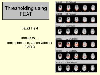
t contrasts • The value of the contrast in each voxel is divided by an estimate of the residual variation in the voxel time course (standard error) • produces a t statistic of the contrast • residual variation is based on the raw time course values minus the predicted values from the fitted model • Activation maps (red and yellow blobs superimposed on anatomical images) are produced by mapping the t value at each voxel to a colour • crudely, thresholding is just setting a value of t below which no colour is assigned.
F contrasts • These can be used to find voxels that are active in any one or more of a set of t contrasts • Visual Auditory Tactile 1 -1 0 1 0 -1 • F contrasts are bidirectional (1 -1 also implies -1 1) • rarely a good thing in practice….. • If the response to an event was modelled with the standard HRF regressor plus time derivative then you can use an F contrast to view both components of model of the response to the event on a single activation map • If you are relying on the time derivative to deal with slice timing correction then you are strongly advised to do this
Temporal autocorrelation • The image intensity value in a voxel at time X is partially predictable from the same voxel at times X-1, X-2, X-3 etc (even in baseline scans with no experiment) • why is this a problem? • it makes it hard to know the number of statistically independent observations in a voxel time course • life would be simple if the number of observations was equal to the number of functional volumes • temporal autocorrelation results in a true N is lower than this • Why do we need to know the number of independent observations? • because calculating a t statistic requires dividing by the standard error, and the standard error is SD / square root (N-1) • Degrees of freedom are needed to convert t stats to p values • If you use the number of time points in the voxel time course as N then p values will be too small (false positive)
Temporal autocorrelation • Generally, the value of a voxel at time t is partially predictable from nearby time points about 3-6 seconds in the past • So, if you use a very long TR, e.g. 6, then you mostly avoid the problem as the original time points will have sufficient independence from each other • Voxel values are also predictable from more distant time points due to low frequency noise with periodic structure • but the high pass filter should deal with this problem
Autocorrelation: FILM prewhitening • First, fit the model (regressors of interest and no interest) to the voxel time course using the GLM • (ignoring the autocorrelation for the moment) • Estimate the temporal autocorrelation structure in the residuals • note: if model is good residuals = noise? • The estimated structure can be inverted and used as a temporal filter to undo the autocorrelation structure in the original data • the time points are now independent and so N = the number of time points (volumes) • the filter is also applied to the design matrix • Refit the GLM • Run t and F tests with valid standard error and degrees of freedom • Prewhitening is selected on the stats tab in FEAT • it is computationally intensive, but with a modern PC it is manageable and there are almost no circumstances where you would turn this option off
Spatial smoothing • FMRI noise varies across space as well as time • smoothing is a way of reducing spatial noise and thereby increasing the ratio of signal to noise (SNR) in the data • Unlike FMRI temporal noise, FMRI spatial noise is more like white noise, making it easier to deal with • it is essentially random, essentially independent from voxel to voxel, and has as mean of about zero • therefore if you average image intensity across several voxels, noise tends to average towards zero, whereas signal that is common to the voxels you are averaging across will remain unchanged, dramatically improving the signal to noise ratio (SNR) • A secondary benefit of smoothing is to reduce anatomical variation between participants that remains after registration to the template image • this is because smoothing blurs the images
Spatial smoothing: FWHM • FSL asks you to specify a Gaussian smoothing kernel defined by its Full Width at Half Maximum (FWHM) in mm • To find the FWHM of a Gaussian • Find the point on the y axis where the function attains half its maximum value • Then read off the corresponding x axis values
Spatial smoothing: FWHM • The Gaussian is centred on a voxel, and the value of the voxel is averaged with that of adjacent voxels that fall under the Gaussian • The averaging is weighted by the y axis value of the Gaussian at the appropriate distance
No smoothing 4 mm 9 mm