Reconnaissance d’objets et vision artificielle

Reconnaissance d’objets et vision artificielle 2009 Reconnaissance d’objets et vision artificielle Josef Sivic http://www.di.ens.fr/~josef Equipe-projet WILLOW, ENS/INRIA/CNRS UMR 8548 Laboratoire d’Informatique, Ecole Normale Supérieure, Paris

Plan for the reminder of the class today • Assignments • 2. Brief review of linear filtering • 3. Efficient indexing for visual search and recognition of particular objects

Admin Stuff • Mailing list for the class • - Please write your name and email address • - Will be used to distribute class announcements

Assignments • Due date for assignment 1 (Scale-invariant blob detection) postponed to next week (Nov. 3rd). • Assignment 2: Stitching photo-mosaics out. Note that due date is still two weeks from now (Nov. 10th). • See the course webpage: • http://www.di.ens.fr/willow/teaching/recvis09/

Assignment 2: Stitching photo-mosaics

Assignments • Due date for assignment 1 (Scale-invariant blob detection) postponed to next week (Nov. 3rd). • Assignment 2: Stitching photo-mosaics out. Note that due date is still two weeks from now (Nov. 10th). • http://www.di.ens.fr/willow/teaching/recvis09/ • Any questions?

Linear filtering – brief review With slides from: S. Lazebnik and others

Motivation I.: Blob detection • Assignment I.: Scale-invariant blob detection using the Laplacian of Gaussian filter • filt_size = 2*ceil(3*sigma)+1; % filter size • LoG = sigma^2 * fspecial('log', filt_size, sigma); • imFiltered = imfilter(im, LoG, 'same', 'replicate');

Motivation II: Noise reduction • Given a camera and a still scene, how can you reduce noise? Take lots of images and average them! What’s the next best thing? Source: S. Seitz

1 1 1 1 1 1 1 1 1 “box filter” Moving average • Let’s replace each pixel with a weighted average of its neighborhood • The weights are called the filter kernel • What are the weights for a 3x3 moving average? Source: D. Lowe

f Defining convolution • Let f be the image and g be the kernel. The output of convolving f with g is denoted f * g. • Convention: kernel is “flipped” • MATLAB: conv2 vs. filter2 (also imfilter) Source: F. Durand

Key properties • Linearity: filter(f1 + f2 ) = filter(f1) + filter(f2) • Shift invariance: same behavior regardless of pixel location: filter(shift(f)) = shift(filter(f)) • Theoretical result: any linear shift-invariant operator can be represented as a convolution Source: S. Lazebnik

Properties in more detail • Commutative: a * b = b * a • Conceptually no difference between filter and signal • Associative: a * (b * c) = (a * b) * c • Often apply several filters one after another: (((a * b1) * b2) * b3) • This is equivalent to applying one filter: a * (b1 * b2 * b3) • Distributes over addition: a * (b + c) = (a * b) + (a * c) • Scalars factor out: ka * b = a * kb = k (a * b) • Identity: unit impulse e = […, 0, 0, 1, 0, 0, …],a * e = a Source: S. Lazebnik

Annoying details • What is the size of the output? • MATLAB: filter2(g, f, shape) • shape = ‘full’: output size is sum of sizes of f and g • shape = ‘same’: output size is same as f • shape = ‘valid’: output size is difference of sizes of f and g full same valid g g g g f f f g g g g g g g g Source: S. Lazebnik

Annoying details • What about near the edge? • the filter window falls off the edge of the image • need to extrapolate • methods: • clip filter (black) • wrap around • copy edge • reflect across edge Source: S. Marschner

Annoying details • What about near the edge? • the filter window falls off the edge of the image • need to extrapolate • methods (MATLAB): • clip filter (black): imfilter(f, g, 0) • wrap around: imfilter(f, g, ‘circular’) • copy edge: imfilter(f, g, ‘replicate’) • reflect across edge: imfilter(f, g, ‘symmetric’) Source: S. Marschner

0 0 0 0 1 0 0 0 0 Practice with linear filters ? Original Source: D. Lowe

0 0 0 0 1 0 0 0 0 Practice with linear filters Original Filtered (no change) Source: D. Lowe

0 0 0 0 0 1 0 0 0 Practice with linear filters Original Shifted left By 1 pixel Source: D. Lowe

1 1 1 1 1 1 1 1 1 Practice with linear filters Original Blur (with a box filter) Source: D. Lowe

0 1 0 1 1 0 1 0 1 2 1 0 1 0 1 0 1 0 Practice with linear filters - ? (Note that filter sums to 1) Original Source: D. Lowe

0 1 0 1 1 0 1 0 1 2 1 0 1 0 1 0 1 0 Practice with linear filters - Original • Sharpening filter • Accentuates differences with local average Source: D. Lowe

Sharpening Source: D. Lowe

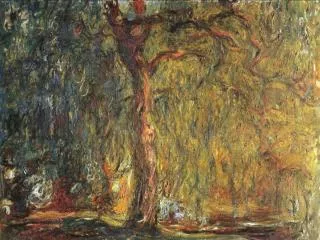
Smoothing with box filter revisited • Smoothing with an average actually doesn’t compare at all well with a defocused lens • Most obvious difference is that a single point of light viewed in a defocused lens looks like a fuzzy blob; but the averaging process would give a little square Source: D. Forsyth

Smoothing with box filter revisited • Smoothing with an average actually doesn’t compare at all well with a defocused lens • Most obvious difference is that a single point of light viewed in a defocused lens looks like a fuzzy blob; but the averaging process would give a little square • Better idea: to eliminate edge effects, weight contribution of neighborhood pixels according to their closeness to the center, like so: “fuzzy blob” Source: S. Lazebnik

Gaussian Kernel • Constant factor at front makes volume sum to 1 (can be ignored, as we should re-normalize weights to sum to 1 in any case) 0.003 0.013 0.022 0.013 0.003 0.013 0.059 0.097 0.059 0.013 0.022 0.097 0.159 0.097 0.022 0.013 0.059 0.097 0.059 0.013 0.003 0.013 0.022 0.013 0.003 5 x 5,  = 1 Source: C. Rasmussen

Choosing kernel width • Gaussian filters have infinite support, but discrete filters use finite kernels Source: K. Grauman

Choosing kernel width • Rule of thumb: set filter half-width to about 3 σ Source: S. Lazebnik

Example: Smoothing with a Gaussian Source: S. Lazebnik

Mean vs. Gaussian filtering Source: S. Lazebnik

Gaussian filters • Remove “high-frequency” components from the image (low-pass filter) • Convolution with self is another Gaussian • So can smooth with small-width kernel, repeat, and get same result as larger-width kernel would have • Convolving two times with Gaussian kernel of width σ is same as convolving once with kernel of width σ√2 • Separable kernel • Factors into product of two 1D Gaussians Source: K. Grauman

Separability of the Gaussian filter Source: D. Lowe

* = = * Separability example 2D convolution(center location only) The filter factorsinto a product of 1Dfilters: Perform convolutionalong rows: Followed by convolutionalong the remaining column: Source: K. Grauman

Separability • Why is separability useful in practice? • Assignment 1: • Is the Laplacian of Gaussian filter separable?

Reconnaissance d’objets et vision artificielle