Download
1 / 35
680 likes | 1.73k Views
Neural Networks Lecture 4 Least Mean Square algorithm for Single Layer Network. Dr. Hala Moushir Ebied. Faculty of Computers & Information Sciences Scientific Computing Department Ain Shams University. Outline. Going back to Perceptron Learning rule

E N D
Neural NetworksLecture 4Least Mean Square algorithm for Single Layer Network Dr. Hala Moushir Ebied Faculty of Computers & Information Sciences Scientific Computing Department Ain Shams University
Outline • Going back to Perceptron Learning rule • Adaline (Adaptive Linear Neuron) Networks • Derivation of the LMS algorithm • Example • Limitation of Adaline
Going back to Perceptron Learning rule • The Perceptronis presented by Frank Rosenblatt (1958, 1962) • The Perceptron, is a feedforward neural network with no hidden neurons. The goal of the operation of the perceptron is to learn a given transformation using learning samples with input x and corresponding output y = f (x). • It uses the hard limit transfer function as the activation of the output neuron. Therefore the perceptron output is limited to either 1 or –1.
Perceptron network Architecture • The update of the weights at iteration n+1 is: Wkj(n+1) = wkj (n)+ wkj (n) Since:
Limit of Perceptron Learning rule • If there is no separating hyperplane, the perceptron will never classify the samples 100% correctly. • But there is nothing from trying. So we need to add something to stop the training, like: • Put a limit on the number of iterations, so that the algorithm will terminate even if the sample set is not linearly separable. • Include an error bound. The algorithm can stop as soon as the portion of misclassified samples is less than this bound. This ideal is developed in the Adaline training algorithm.
Error Correcting Learning • The objective of this learning is to start from an arbitrary point error and then move toward a global minimum error, in a step-by-step fashion. • The arbitrary point error determined by the initial values assigned to the synaptic weights. • It is closed-loop feedback learning. • Examples of error-correction learning: • the least-mean-square (LMS)algorithm (Windrow and Hoff), also called delta rule • and its generalization known as the back-propagation (BP) algorithm.
Outline • Learning Methods: • Adaline (Adaptive Linear Neuron) Networks • Derivation of the LMS algorithm • Example • Limitation of Adaline
Adaline (Adaptive Linear Neuron) Networks • 1960 - Bernard Widrow and his student Marcian Hoff introduced the ADALINE Networks and its learning rule which they called the Least mean square (LMS) algorithm (or Widrow-Hoff algorithm or delta rule) • The Widrow-Hoff algorithm • can only train single-Layer networks. • Adaline similar to the perceptron, the differences are ….? • Both the Perceptron and Adaline can only solve linearly separable problems • (i.e., the input patterns can be separated by a linear plane into two groups, like AND and OR problems).
Adaline Architecture • Given: • xk(n): an input value for a neuron k at iteration n, • dk(n): the desired response or the target response for neuron k. • Let: • yk(n) : the actual response of neuron k.
ADALINE’s Learning as a Search • Supervised learning: {p1,d1}, {p2,d2},…,{pn,dn} • The task can be seen as a search problem in the weight space: • Start from a random position (defined by the initial weights) and find a set of weights that minimizes the error on the given training set
The error function: Mean Square Error • ADALINEs use the Widrow-Hoff algorithm or Least Mean Square (LMS) algorithm to adjusts the weights of the linear network in order to minimize the mean square error • Error : difference between the target and actual network output (delta rule). error signal for neuron k at iteration n: ek(n) = dk(n)- yk(n)
Error Landscape in Weight Space • Total error signal is a function of the weights • Ideally, we would like to find the global minimum (i.e. the optimal solution) E(w) Decreasing E(w) w1 E(w) Decreasing E(w) w1
Error Landscape in Weight Space, cont. • The error space of • the linear networks (ADALINE’s) is a parabola (in 1d: one weight vs. error) or • a paraboloid (in high dimension) • and it has only one minimum called the global minmum.
(w1,w2) (w1+w1,w2 +w2) Error Landscape in Weight Space, cont. • Takes steps downhill • Moves down as fast as possible • i.e. moves in the direction that makes the largest reduction in error • how is this direction called?
Steepest Descent • The direction of the steepest descent is called gradientand can be computed • Any function increases most rapidly when the direction of the movement is in the direction of the gradient • Any function decreases most rapidly when the direction of movement is in the direction of the negative of the gradient • Change the weightsso that we move a short distance in the direction of the greatest rate of decrease of the error, i.e., in the direction of –vegradient. Dw = - η * E/w
Outline • Learning Methods: • Going back to, Perceptron Learning rule and its limit • Error Correcting Learning • Adaline (Adaptive Linear Neuron Networks) Architecture • Derivation of the LMS algorithm • Example • Limitation of Adaline
The Gradient Descent Rule • It consists of computing the gradient of the error function, then taking a small step in the direction of negative gradient, which hopefully corresponds to decrease function value, then repeating for the new value of the dependent variable. • In order to do that, we calculate the partial derivative of the error with respect to each weight. • The change in the weight proportional to the derivative of the error with respect to each weight, and additional proportional constant (learning rate) is tied to adjust the weights. Dw = - η * E/w
LMS Algorithm - Derivation • Steepest gradient descent rule for change of the weights: Given • xk(n): an input value for a neuron k at iteration n, • dk(n): the desired response or the target response for neuron k. Let: • yk(n) : the actual response of neuron k. • ek(n) : error signal = dk(n)- yk(n) Train the wi’s such that they minimize the squared error after each iteration
LMS Algorithm – Derivation, cont. • The derivative of the error with respect to each weight can be written as: • Next we use the chain rule to split this into two derivatives:
LMS Algorithm – Derivation, cont. • This is called the Delta Learning rule. • Then • The Delta Learning rule can therefore be used Neurons with differentiable activation functions like the sigmoid function.
LMS Algorithm – Derivation, cont. • The widrow-Hoff learning rule is a special case of Delta learning rule. Sincethe Adaline’s transfer function is linear function: • then • The widrow-Hoff learning rule is:
Adaline Training Algorithm 1- initialize the weights to small random values and select a learning rate, (h) 2-Repeat 3- form training patterns select input vector X , with target output, t, compute the output: y = f(v), v = b + wTx Compute the output error e=t-y update the bias and weights wi (new) = wi (old) + h (t – y ) xi 4- end for 5- untilthe stopping criteria is reached by find the Mean square error across all the training samples stopping criteria: if the Mean Squared Error across all the training samples is less than a specified value, stop the training. Otherwise , cycle through the training set again (go to step 2)
Convergence Phenomenon • The performance of an ADALINE neuron depends heavily on the choice of the learning rate h. • How to choose it? • Too big • the system will oscillate and the system will not converge • Too small • the system will take a long time to converge • Typically, h is selected by trial and error • typical range: 0.01 < h < 1.0 • often start at 0.1 • sometimes it is suggested that: 0.1/m < h < 1.0 /mwhere m is the number of inputs • Choose of h depends on trial and error.
Outline • Learning Methods: • Going back to, Perceptron Learning rule and its limit • Error Correcting Learning • Adaline (Adaptive Linear Neuron Networks) Architecture • Derivation of the LMS algorithm • Example • Limitation of Adaline
Example The input/target pairs for our test problem are Learning rate: h = 0.4 Stopping criteria: mse < 0.03 Show how the learning proceeds using the LMS algorithm?
Example Iteration One First iteration – p1 e = t – y = -1 – 0 = -1
Example Iteration Two Second iteration – p2 e = t – y = 1 – (-0.4) = 1.4 End of epoch 1, check the stopping criteria
Example – Check Stopping Criteria For input P1 For input P2 Stopping criteria is not satisfied, continue with epoch 2
Example – Next Epoch (epoch 2) Third iteration – p1 e = t – y = -1 – 0.64 = -0.36 if we continue this procedure, the algorithm converges to: W(…) = [1 0 0]
Outline • Learning Methods: • Adaline (Adaptive Linear Neuron Networks) Architecture • Derivation of the LMS algorithm • Example • Limitation of Adaline
ADALINE Networks - Capability and Limitations • Both ADALINE and perceptron suffer from the same inherent limitation - can only solve linearly separable problems • LMS, however, is more powerful than the perceptron’s learning rule: • Perceptron’s rule is guaranteed to converge to a solution that correctly categorizes the training patterns but the resulting network can be sensitive to noiseas patterns often lie close to the decision boundary • LMS minimizes mean square error and therefore tries to move the decision boundary as far from the training patterns as possible • In other words, if the patterns are not linearly separable, i.e. the perfect solution does not exist, an ADALINE will find the best solution possible by minimizing the error (given the learning rate is small enough)
Comparison with Perceptron • Both use updating rule changing with each input • One fixes binary error; the other minimizes continuous error • Adaline always converges; see what happens with XOR • Both can REPRESENT Linearly separable functions • The Adaline, is similar to the perceptron, but their transfer function is linear rather than hard limiting. This allows their output to take on any value.
Summary • ADALINE Like perceptrons: • ADALINE can be used to classify objects into 2 categories • it can do so only if the training patterns are linearly separable • Gradient descent is an optimizationalgorithm that approaches a local minimum of a function by taking steps proportional to the negative of the gradient (or the approximate gradient) of the function at the current point. If instead one takes steps proportional to the gradient, one approaches a local maximum of that function; the procedure is then known as gradient ascent. • Gradient descent is also known as steepest descent, or the method of steepest descent.