Download
1 / 31
320 likes | 484 Views
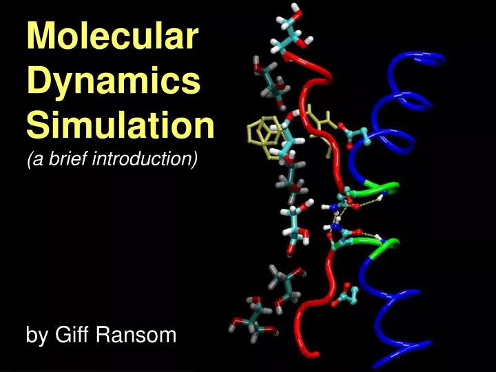
Molecular Dynamics Simulation (a brief introduction). by Giff Ransom. A Digital Laboratory.

E N D
Molecular Dynamics Simulation(a brief introduction) by Giff Ransom
A Digital Laboratory “In the real world, this could eventually mean that most chemical experiments are conducted inside the silicon of chips instead of the glassware of laboratories. Turn off that Bunsen burner; it will not be wanted in ten years.” - The Economist, reporting on the work of the 1998 Chemistry Nobel Prize Awardees
A Different Type of Simulation • Many Physically-Based Simulations model easily observable real world phenomena. • Molecular Dynamics Simulations model things too small for us to observe directly.
Why Not Quantum Mechanics? • Modeling the motion of a complex molecule by solving the wave functions of the various subatomic particles would be accurate… • But it would also be very hard to program and take more computing power than anyone has!
Classical Mechanics • Instead of using Quantum mechanics, we can use classical Newtonian mechanics to model our system. • This is a simplification of what is actually going on, and is therefore less accurate. • To alleviate this problem, we use numbers derived from QM for the constants in our classical equations.
Molecular Modeling For each atom in every molecule, we need: • Position (r) • Momentum (m + v) • Charge (q) • Bond information (which atoms, bond angles, etc.)
From Potential to Movement To run the simulation, we need the force on each particle. We use the gradient of the potential energy function. Now we can find the acceleration.
What is the Potential? A single atom will be affected by the potential energy functions of every atom in the system: • Bonded Neighbors • Non-Bonded Atoms (either other atoms in the same molecule, or atoms from different molecules)
Non-Bonded Atoms There are two potential functions we need to be concerned about between non-bonded atoms: • van der Waals Potential • Electrostatic Potential
The van der Waals Potential • Atoms with no net electrostatic charge will still tend to attract each other at short distances, as long as they don’t get too close. • Once the atoms are close enough to have overlapping electron clouds, they will repel each other with astounding force
The van der Waals Potential One of the most widely used functions for the van der Waals potential is the Lennard-Jones. It is a compromise between accuracy and computability.
The van der Waals Potential The Constants A and C depend on the atom types, and are derived from experimental data.
The Electrostatic Potential • Opposite Charges Attract • Like Charges Repel • The force of the attraction is inversely proportional to the square of the distance
The Non-Bonded Potential Combine the LJ and Electrostatic Potentials
Bonded Atoms There are three types of interaction between bonded atoms: • Stretching along the bond • Bending between bonds • Rotating around bonds
Bond Length Potentials Both the spring constant and the ideal bond length are dependent on the atoms involved.
Bond Angle Potentials The spring constant and the ideal angle are also dependent on the chemical type of the atoms.
Torsional Potentials Described by a dihedral angle and coefficient of symmetry (n=1,2,3), around the middle bond.
Integration Algorithms • Forces like the LJ potential have powers of 12, which would make Euler horribly unstable (even worse than usual) • RK and Midpoint algorithms would seem to help • However, force calculations are extremely expensive, and RK and Midpoint require multiple force calculations per timestep
Integration Algorithms • Using RK is justifiable in other circumstances, because it allows you to take larger timesteps (two force calculations allowing you to more than double the timestep) • This is normally not achievable in MD simulations, because the forces are very rapidly changing non-linear functions. • We need an algorithm with the stability benefits of RK without the cost of extra force calculations!
Verlet Algorithm • First, take a third-order Taylor step: • Now take a step backward:
Verlet Algorithm • When adding the two formulas, the first and third derivatives cancel out: • And we can express the next timestep in terms of the previous position and the current acceleration:
Verlet Algorithm Pros: • Simple & Effective • Low Memory & CPU Requirements (don’t need to store velocities or perform multiple force calculations) • Time Reversible • Very stable even with large numbers of interacting particles Cons: • Not as accurate as RK • We never calculate velocities! (when would we need them?)
Obtaining Velocities • We can estimate the velocities using a finite difference: • This has a second order error, while our algorithm has a fourth order error • There are variations of the Verlet algorithm, such as the leapfrog algorithm, which seek to improve velocity estimations.
Molecules in Solution • In real situations, a molecule is rarely isolated. In biological systems, proteins, RNA, and DNA are immersed in a sea of water molecules • To accurately portray the effect of the solvent molecules on a system, the solvent molecules must be free flowing • How do we establish computational boundaries while keeping a realistic solvent simulation?
Periodic Boundary Conditions • Simulate a segment of molecules in a larger solution by having repeatable regions • Potential calculations are run only on each atom’s closest counterpart in the 27 cubes • When an atom moves off the edge, it reappears on the other side (like in asteroids)
Cutoff Methods • Ideally, every atom should interact with every other atom • This creates a force calculation algorithm of quadratic order • We may be able to ignore atoms at large distances from each other without suffering too much loss of accuracy
Cutoff Methods • Truncation – cuts off calculation at a predefined distance • Shift – alters the entire function as to be zero at the cutoff distance • Switch – begins tapering to zero as the function approaches the cutoff distance
Live Demo Using NAMD (Not Another Molecular Dynamics Simulation) and VMD (Visual Molecular Dynamics) from the University of Illinois at Urbana Champaign
Resources Books • Tamar Schlick Molecular Modeling and Simulation: An Interdisciplinary Guide2002 • Alan Hinchliffe Molecular Modelling for Beginners 2003 • D. C. Rapaport The Art of Molecular Dynamics Simulation.2004 • Daan Frenkel, B. Smit Understanding Molecular Simulation2001 Websites • Molecular Dynamics Tutorial at EMBnethttp://www.ch.embnet.org/MD_tutorial/index.html • Theoretical and Computational Biophysics Group at UIUC (home of VMD and NAMD)http://www.ks.uiuc.edu/