Download
1 / 14
140 likes | 204 Views
What happens to detailed balance away from equilibrium?. R. M. L. Evans University of Leeds School of Physics & Astronomy. Driven steady states. g. Semi- dilute “living” polymers. A phase of amphiphiles. s. ...self-assembled into “worm-like micelles”:. Stirring causes de-mixing!.

E N D
What happens to detailed balance away from equilibrium? R. M. L. Evans University of Leeds School of Physics & Astronomy
Driven steady states g Semi- dilute “living” polymers A phase of amphiphiles... s ...self-assembled into “worm-like micelles”: Stirring causes de-mixing! Driven steady states are not at thermodynamic equilibrium because, by definition, equilibrium states have no net fluxes. Examples:Fluids under shear Particularly interesting for complex fluids, where typical relaxation times t are long, so can reach the regime
Lamellar phase of amphiphiles ... into the onion phase: Useful for encapsulating drugs. ...re-structure under shear
Any concentrated suspension Traffic e.g. O. O’Loan & M. R. Evans ’97: Re-structures, under sufficiently high shear, into force-bearing chains... + spectator particles.
Compare equilibrium states with driven states Equilib. states Driven states Ubiquitous. Well-defined statisticallysteady states in dynamic systems with spatial and temporal fluctuations. Have transitions between differently-structured states at well-defined values of the control parameters. Exhibit phase transition in 1 dimension. We can use intuition and approximation to model them mathematically. We understand the universal statistical principles underlying their behaviour, and respect those principles when constructing models.
Current approaches to non-equilibrium systems (i) Near-equilibrium approximations Assume free energy F(f) can still be defined at non-equilibrium values of order parameter f, and postulate dynamics, e.g. —“Model A” for non-conserved O.P. Implies local coarse-graining. (ii) Invent microscopic dynamics ...and derive the macroscopic consequences. e.g. The bus route model: This is fine, but it’s not how we do things at equilibrium, where rates cannot be chosen entirely arbitrarily, but must obey the principle of detailed balance, to respect Boltzmann. i.e. Macroscopic thermodynamics informs the microscopic model.
Where does Detailed Balance come from? c c a b • If Ea=Eb then wab=wba. • So DB embodies reversibility. • DB says something about how likely it is forthe reservoir to give a particular kick to the system. • i.e. It is making a statement about the statistics of the reservoir: that the reservoir is in the most likely state for the given energy. Is it necessarily right?NO! The reservoir might contain anything.
If : (i) system and reservoir have reversible microscopic dynamics (ii) system and reservoir are in an ergodic steady state (exploring phase space thoroughly) (iii) reservoir is characterised only by its macroscopic observables (energy) i.e. is in the most likely statistical state with no surprises then the rates are constrained to respect detailed balance ( N/2 constraints on the N rates wab ). Take such a system+reservoir, and subject it to continuous shear. All 3 above conditions continue to be true. Are we free to choose rates arbitrarily in every non-equilib model? No! Those 3 conditions lead to N/2 constraints. i.e. There must be a non-equilibrium counterpart to the principle of detailed balance.
Driven steady-state ensemble Dg system N h >> lcorr Statistical weight of ensemble is no. of ways of permuting these differently-experienced systems: ... system 2 By definition, most ensembles maximise the statistical weight. This is achieved by maximising (subject to constraints) system 1 Imagine a large set of fluid systems stacked up and sheared: (e.g. fluid is the onion phase of amphiphiles) Over a long duration t, system i follows path Gi through phase space. We derive the path distribution pG following Gibbs: Number of systems with trajectory G is nG=NpG
Recipe To find distribution pG of phase-space paths (drawn only from the set of physically possible paths), • maximise ‘path entropy’ Swith respect topG, subject to constraints: • Normalization, • Known macroscopic observables, (equilib.) • Extra constraint on driven ensemble: Result: • NB This is a well known recipe (proposed by Jaynes), but: • is normally wrapped up with unsatisfactory subjective (Bayesian/information-theoretic) interpretation of probabilities; defined here in terms of concrete countable quantities. • is often considered unhelpful, or used only approximately, because G is a high-dimensl. object. We’ll use it to find rates wab.
Implications for rates b Would like to know prob. of a particular transition a→b, to find state a time By counting all paths that contain this transition, the relation between and implies: We are not entirely free to choose since detailed balance must be respected. Hence, are subject to the same amount of constraint. Example: Hopping in 1D Macro-observable: where G(x,t) is equilib Green’s fn. L R 0 x and We have the probability of an entire path G:
Activated processes Simple model:
Overview • Postulated some exactrules for: • microscopically reversible • ergodic steady states • with uncorrelated (i.e. weakly coupled) reservoir. • Like detailed balance, rules do not fully specify rates. • Results are only as good as the chosen model: should include momentum variables. Further work • Aditi Simha has found rules yield interactions, in many-particle systems, that respect Newton’s 3rd law. • Adrian Baule will test rules by modelling real systems. Thanks to: Peter Olmsted, Richard Blythe, Mike Cates, Alistair Bruce, Tom McLeish.