Download
1 / 20
250 likes | 511 Views
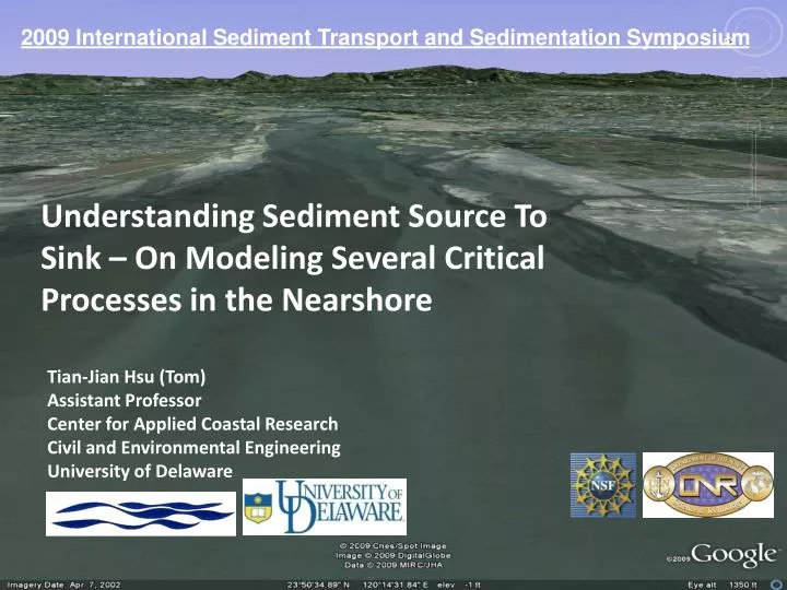
2009 International Sediment Transport and Sedimentation Symposium. Understanding Sediment Source To Sink – On Modeling Several Critical Processes in the Nearshore. Tian-Jian Hsu (Tom) Assistant Professor Center for Applied Coastal Research Civil and Environmental Engineering

E N D
2009 International Sediment Transport and Sedimentation Symposium Understanding Sediment Source To Sink – On Modeling Several Critical Processes in the Nearshore Tian-Jian Hsu (Tom) Assistant Professor Center for Applied Coastal Research Civil and Environmental Engineering University of Delaware
Fate of Terrestrial Sediment in Coastal Ocean (Sediment source to sink) - Why is it important? • Coastal Ecosystem • Heath of coral reef • Contaminant Transport • Carbon Sequestration • Yes, sediment transport is • related to Global Warming! • Particulate Organic Carbon and • nutrients are carried by river • borne sediments. • Seabed Properties • They determine surface wave • propagation and acoustic wave • transmission. • Waterway Navigation • dredging In “Mud, Marine Snow and Coral Reefs” by Eric Wolanski, Robert Richmond, Laurence McCook and Hugh Sweatman, American Scientist, 91 (1), p. 44. Adopted from MARGINS Science Plans 2004. National Science Foundation. A soft mud bed at a tidal flat in Willapa Bay, WA
Where are the big signals? Large rivers in passive margin – Amazon, Mississippi Small mountainous river in active margin – e.g., Kaoping (Taiwan), Jhoushui (Taiwan), Waipaoa (New Zealand), Santa Clara and Eel (USA). See Milliman & Syvitski (1992) J. Geology. Adopted from MARGINS Science Plans 2004. National Science Foundation.
Physical Settings of Small Mountainous River • Episodic high sediment yield triggered by large rainfall due to typhoon or • tropic cyclone (sediment concentration often exceeding several g/l). • Highly salt-stratified frontal zone. • Energetic wave condition. ROMS model results for highly sal-stratified frontal zone adopted from Hetland & MacDonald (2008) Spreading in the near-field Merrimack River plume, Ocean Modeling, 21, 12-21. Left: SAR image of Jhoushui river mouth courtesy of Dr. Chang at Center for Space & Remote Sensing Research, National Central Univ., Taiwan. Right: Figures of Landslides and river flooding after typhoon Mindulle (July 2005) are provided by Dr. S.-J. Kao, Academia Sinica, Taiwan.
Motivation Large-scale coastal models, e.g. Delft3D, MIKE21, NOPP-CSTMS (ROMS), ECOMSED (POMS) and many others, require accurate parameterization on small-scale processes. NOPP-CSTMS (Community Sediment Transport Model System): CSTMS model results provided by Chris Sherwood (USGS) and Rocky Geyer (WHOI). http://www.cstms.org Wave boundary layer process and near-bed sediment transport require grid resolution ~ 1 mm Frontal dynamics requires grid resolution ~ cm ~10m ~20cm
z dilute turbulent suspension < o lutocline mobile fluid mud o < < gel Consolidating bed > gel ~10g/l ~100g/l Fluid Mud Modeling Develop a numerical modeling framework for fine sediment transport based on Fast Equilibrium Eulerian Approximation (Ferry & Balachandar 2001) to the Eulerian Two-phase formulation – Mixture Approach • Mass and momentum equations: • Turbulent & viscous stresses; rheological stresses. • Sediment-driven gravity flow. • Turbulence closure: damping of turbulence due to sediment density stratification and viscous drag in turbulent fluctuation. • Rheological stress: e.g., Bingham-plastic. Important to hydrodynamic dissipation. • Floc properties and floc dynamics assuming fractal structure. Winterwerp (1998), Khelifa & Hill (2006), Son & Hsu (2008). • Erodibility (Type I erosion): critical bottom stress depends on cumulative eroded mass. • Future work: Directly resolve bed consolidation and fluidization (e.g., Gibson et al. 1967). Evolution of floc aggregate structure. Winterwerp & van Kesteren (2004)
Numerical Implementation • 2DV turbulence-averaged fine sediment modeling framework is solved numerically by revising a 2DV time/depth resolving wave model (COBRAS, Lin and Liu 1998, JFM). A non-hydrostatic 2D RANS solver with complex bathymetry. • COBRAS can calculate surface wave propagation using volume of fluid (VOF) scheme and is a powerful tool for nearshore where wave effects are important. • When sediment concentration and salinity 0, numerical model reduces to original COBRAS for clear fluid RANS model. Model results on surf zone wave provided by Alec Torres-Freyermuth, CACR, U. Delaware.
Wright & Nittrouer [1995], Estuaries. App #1: Sediment-laden River Plume & Initial Deposition • Positively Buoyant Plume (~<40g/l): • Frontal trapping, lift-off, etc (e.g., Armi & Farmer 1986; Geyer & Kineke 1995; Wu et al. 2006; Lee et al. 2009). • Sediment settling (Hill et al. 2000): • Primary particle (↓ 0.1 mm/s) • Flocculation process(↓ 1 mm/s) • Convective sedimentation (↓ 1 cm/s) • (e.g., Green 1987; • Parson, Bush & Syvitski 2001; • McCool & Parson 2004) • Negatively Buoyant Plume: (>40g/l) • Hyperpycnal flow (Wright et al. 1988, Nature, vol. 332, p. 629) • Buoyancy reversal (due to rapid sediment deposition, Hurzeler et al. 1996; Hogg et al. 1999)
Hyperpycnal plume – silt River discharge, U0=20 cm/s, cin=47 g/l, Salinity of seawater 35 ppt, ccric=42 g/l Silt: d=20 µm, s=2650 kg/m3, Ws=0.36 mm/s Salinity (ppt) Sed. conc. (g/l)
Hypopycnal plume (convective sed.)– silt, clay (primary particle) River discharge, U0=20 cm/s, cin=26.5 g/l, Salinity of seawater 35 ppt, ccric=42 g/l Silt: d=20 µm, s=2650 kg/m3, Ws=0.36 mm/s Salinity (ppt) Sed. conc. (g/l)
Convective Sedimentation/Instability • Earlier studies explain this phenomenon based on double-diffusion analogy for salt-finger:e.g., Green (1987), Sedimentology; Chen, (1997) Deep-Sea Research; Hoyal, Bursik, and Atkinson (1999) Marine Geology. • McCool & Parsons (2004) carry out first experiment for convective instability with ambient shear flow. They observe convective instability with sediment concentration as low as 380mg/l. Parsons, Bush, Syvitski,, 2001, Sedimentology, 48, 465-478. Science Issue #1: Is double-diffusion the only explanation of convective instability? How about gravitational settling itself? McCool & Parsons, 2004, Cont. Shelf Res., 24, 1129-1142.
Sicence Issue #2: Can convective instability occur in the field? Recent field study by Warrick et al. (2008, Cont. Shelf Res.) at Santa Clara River, CA observe rapid sediment settling from bottom tripod, which was indirectly related to convective instability (not direct field evidence). Our numerical model results suggest when inlet height is larger (~meters), strong interfacial mixing (K-H waves, Holmboe waves) can suppress convective instability: It is likely that convective instability can occur in the field but with much larger sediment concentration, i.e., 10~20 g/l. Important for small mountainous river. This problem is strongly related to plume dynamics (e.g., hydraulic control, Armi and Farmer 1986), and interfacial mixing. What is the effect of surface gravity waves?
Resuspension • Currents (tidal-, wind-driven, etc) and waves can suspend high concentration cohesive sediment – Fluid mud • Wave dissipation over mud. • Wave-supported gravity-driven mudflows (e.g., Ogston et al. 2000; Traykovski et al 2000; Wright et al. 2001). Adopted from MARGINS Science Plans 2004. National Science Foundation. Traykovski et al. [2000], Cont. Shelf Res.
App #2: Detailed modeling of wave-supported gravity-driven mudflow and its parameterization(Hsu et al. 2008, JGR - Ocean, accepted). Wright et al. 2001; Marine Geology - Parameterization for coastal modeling 1DV fluid mud model results of wave supported gravity-driven mudflow at Po prodelta. EUROSTRATAFORM data obtained in collaboration with Peter Traykovski (WHOI).
App #3: Wave-mud Interaction – 2DV Modeling The presence of mud can significantly attenuates wave energy (e.g., Gade 1958; Dalrymple & Liu 1978; Sheremet & Stone 2003) Rheological stress closure: Stiffness: kb =>Bingham-type kb=>Newtonian-type
Cnoidal Wave Train Propagating over Muddy Seabed *Numerical modeling of wave-mud interaction is carried out by postdoc Alec Torres-Freyermuth Wave characteristics: H=0.72 m T=6 s L=28 m Mesh characteristics: Min (y)=2 mm Min (x)=2.5 cm Fluid-mud characteristics: D=22 m (floc) f=1340 Kg/m3 nf=2.1 Ws~0.1 mm
Wave Amplitude Dissipation The wave amplitudes present a monotonic decrease in amplitude at various frequency, suggesting both direct interaction (long wave and mud) and wave-wave interaction cause wave attenuation. kh=1 @ x=185 m Clear fluid Fluid mud Clear fluid with increased Ks=400mm Nonlinear wave effects - Ongoing work
Mud-laden Wave Boundary Layer Dynamics (a) Clear fluid (b) Fluid mud
Ongoing and Future Works - related to sediment Disposal off Small Mountainous River • Improved modeling on sediment-laden plume dynamics for high sediment yield condition. • - Small-scale modeling (2DV~1m X 100m); • - Coastal Modeling, e.g., Community Sediment Transport Modeling System (3D ~10m X 5km X 5km) Schematic plot of sediment-laden river plume produced in collaboration with Dr. Rocky Geyer, WHOI
Effects of waves on plume dynamics and sediment deposition (and vice versa) NearCoM Simulation (REF/DIF1+SHORECIRC) 2DV Buoyant plume simulation with free-surface (use VOF scheme): Model results provided by Drs. Fengyan Shi and Jim Kirby University of Delaware. See http://chinacat.coastal.udel.edu/~kirby/programs/nearcom/