Download
1 / 37
390 likes | 601 Views
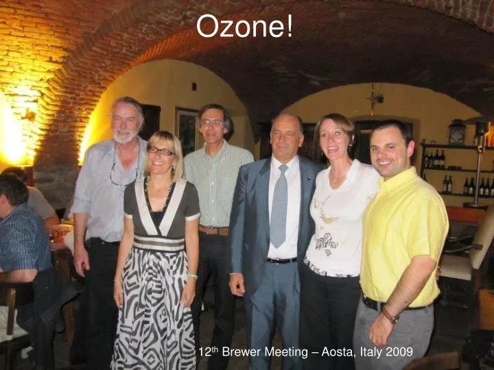
Ozone!. 12 th Brewer Meeting – Aosta, Italy 2009. Introduction to Ozone Measurement. Tom McElroy David Wardle Vladimir Savastiouk. Physical Principles of the Dobson Measurement. Beer’s law 1, 2 Ozone absorption Slant path at 22 km; , m and sec Rayleigh scattering

E N D
Ozone! 12th Brewer Meeting – Aosta, Italy 2009
Introduction to Ozone Measurement Tom McElroy David Wardle Vladimir Savastiouk 13th Biennial Brewer Workshop
Physical Principles of the Dobson Measurement Beer’s law 1, 2 Ozone absorption Slant path at 22 km; , m and sec Rayleigh scattering Langley plots 1, 2 Single wavelength attenuation expression Dobson observations 1, 2 Performance Testing 13th Biennial Brewer Workshop
Handbook Dobson’s Observer’s Handbook 13th Biennial Brewer Workshop
Beer’s Law 1 Cross-section m2 Total optical depth: m2/molecule * molecules / m2 Lost photons: photons / s 13th Biennial Brewer Workshop
Beer’s Law - 2 13th Biennial Brewer Workshop
Beer’s Law - 3 ‘Phenomenological’ 13th Biennial Brewer Workshop
Ozone Absorption - General 13th Biennial Brewer Workshop
Ozone Cross-sections Spectral regions used for ‘optical’ measurements Huggins and Chappuis Cross-sections as Measured in the Laboratory by the GOME FM. GOME- Global Ozone Monitoring Experiment FM – Flight Model 13th Biennial Brewer Workshop
Ozone Absorption - Dobson The tables show the standard Dobson measurement Wavelengths and the optical depths of a 1-cm ozone path. The idea behind both the Dobson and Brewer measurements is that the absolute extinction on a wavelength pair from other things is similar, but the difference in ozone Absorption is large… 13th Biennial Brewer Workshop
Ozone Absorption – Brewer Wavelengths (The small absorption at 324 nm allowed this intensity to be used as a proxy for wavelengths longer than 325 nm in the original short-wavelength-range Brewer UV scans.) 13th Biennial Brewer Workshop
Single-wavelength attenuation expression - 13th Biennial Brewer Workshop
Langley plot: single-wavelength measurement 13th Biennial Brewer Workshop
Differential Measurements 13th Biennial Brewer Workshop
Langley plot – Short and Long Methods 13th Biennial Brewer Workshop
Dobson Observation 13th Biennial Brewer Workshop
Rayleigh scattering 13th Biennial Brewer Workshop
Slant path at 22 km; , m and sec() 13th Biennial Brewer Workshop
Fery Spectrometer 13th Biennial Brewer Workshop
Dobson Spectrophotometer 13th Biennial Brewer Workshop
Brewer Optics ~ 15 cm To Photomultiplier Housing Entrance Slit 13th Biennial Brewer Workshop
Rectifier Phase The Dobson was one of the first opto-electronic instruments to use phase- sensitive detection to improve signal-to-noise ratio and do a direct difference detection. These tracings illustrate the phase setting adjustment made to synchronize the rectifier with the phase of the optical signal. The test is done with a large signal and high signal-to-noise ratio. 13th Biennial Brewer Workshop
Brewer – SH Test • For efficient operation the slits should be open as much as possible (design 7:8) • Only one slit should pass light at one time • Stepping motor must change positions as fast as possible • It must not oscillate when stopped • A non-resonant waveform is generated • The SH test determines the time constant for the waveform 13th Biennial Brewer Workshop
The Brewer – Run/Stop • The Brewer multiplexes rapidly between multiple slits • Photon counting is inhibited while changing slits so the electronics determines the timing interval • The position of the slit mask must change fast with little oscillation to be accurate • The Run/Stop test compares static measurements with dynamic measurements 13th Biennial Brewer Workshop
Measurement Linearity Dobson • Issue largely avoided • Detection of balance only at range of gains • Optical wedge calibrated using 2-source test • ‘N-tables’ used to translate R-values to logs 13th Biennial Brewer Workshop
Linearity - Brewer • Linearity tested explicitly • 2-source test • Done using the DT test • Run with three slit positions • One has 2 slits open at once • Measure: A, B and A&B • Compare: A+B to A&B • Solve for dt in: A = Ao exp( - Ao dt ) B = Bo exp( - Bo dt ) A + B = (Ao + Bo) exp[ - (Ao + Bo) dt ] 13th Biennial Brewer Workshop
Sun Scans 13th Biennial Brewer Workshop
Brewer Sunscan Ozone 13th Biennial Brewer Workshop
The Brewer – SC Test • The solar spectrum is observed under clear conditions (for stability) • The grating angle is scanned by stepping the drive micrometer • An extreme point in the ozone and SO2 is identified near the nominal calibration step • This step position is the calibration point for the instrument (Note that the step number is a function of slant column ozone amount. Traditionally the cal step is chosen near 700 DU slant column ozone amount.) 13th Biennial Brewer Workshop
Ozone v. Step Number 13th Biennial Brewer Workshop
Brewer Calibration • Using direct regression against airmass • Computer-calculated • Station instruments done by comparison to traveling standard Mauna Loa Observatory 13th Biennial Brewer Workshop
Extraterrestrial Constant Lo analysis From Oxford. 13th Biennial Brewer Workshop
Brewer Langley Plot 13th Biennial Brewer Workshop
The Formula… Ozone = (F – Fo) / (mu * alpha) If the ozone is constant, Ozone * alpha = F / mu – Fo / mu Plot F / mu against 1/ mu The slope is Fo 13th Biennial Brewer Workshop
Inverse plot 13th Biennial Brewer Workshop
The End Eureka, Nunavut February 2006