Download
1 / 33
330 likes | 444 Views
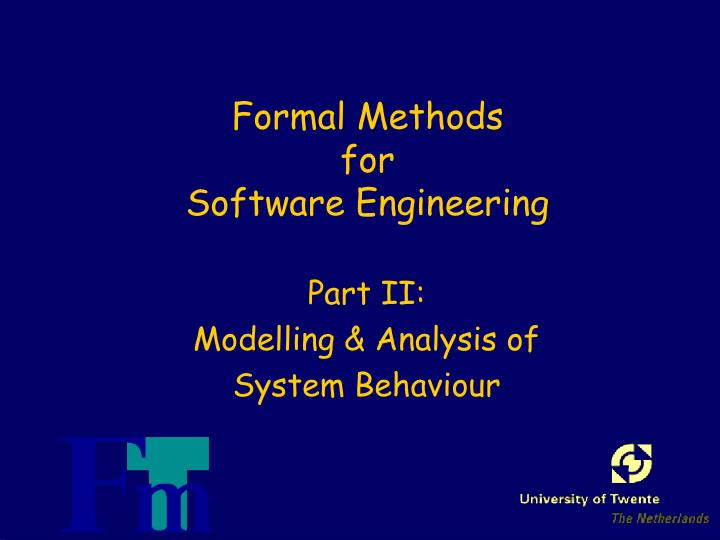
Formal Methods for Software Engineering. Part II: Modelling & Analysis of System Behaviour. Contents Part I. In Part I we used Z as a formalism to model the static aspects of software systems, i.e. definition of system states & data structures definition of operations & preconditions

E N D
Formal Methods for Software Engineering Part II: Modelling & Analysis of System Behaviour
Contents Part I In Part I we used Z as a formalism to model the static aspects of software systems, i.e. • definition of system states & data structures • definition of operations & preconditions The tool Z-Eves was used for specification support and analysis. FMSE, Lecture 4
Contents Part II In this part we introduce FSP as a formalism to model the dynamic aspects of software systems, i.e. • definition of system behaviour (control flow) • definition of control distribution (concurrency) We introduce the tool LTSA for modelling support and analysis. FMSE, Lecture 4
FSP and LTS Models are described using state machines, known as Labelled Transition Systems. These are described textually as Finite State Processes and displayed and analysed by the LTSA analysis tool. • LTS - graphical form • FSP - algebraic form FMSE, Lecture 4
LTS: a definition A labelled transition system T consists of the following ingredients: 1. a set S of states 2. a set L of actions 3. a set ->of transitions of the form s-a->t with s,tS and aL or a=tau 4. an initial state s0 S We also write T=(S,L,->,s0 ). FMSE, Lecture 4
0 1 Modelling Processes A process is modelled as a finite LTS which transits from state to state by executing a sequence of atomic actions. on a light switch LTS off a sequence of actions or trace onoffonoffonoff… FMSE, Lecture 4
in send 0 1 2 getack get 0 1 put A Simple Transmission Protocol SENDER = (in -> send -> getack -> SENDER). rec out RECEIVER = (rec -> out -> ack -> RECEIVER). 0 1 2 ack BUFFER = (get -> put -> BUFFER). FMSE, Lecture 4
in out getack ack Buffer2 Receiver Sender Buffer1 rec send Medium ||MEDIUM = (a:BUFFER||b:BUFFER) /{send/a.get,rec/a.put,ack/b.get,getack/b.put}. ||SYSTEM = (SENDER || MEDIUM ||RECEIVER). Composing the System FMSE, Lecture 4
in send rec out ack 0 1 2 3 4 5 getack The System Behaviour • parallel composition with synchronized communication • equivalent single process can be calculated (with LTSA) FMSE, Lecture 4
Observable Behaviour Observable behaviour abstracts away from internal system actions . in out getack ack Receiver Sender Medium rec send ||SYSTEM = (SENDER||MEDIUM||RECEIVER). FMSE, Lecture 4
System Observable Behaviour Observable behaviour abstracts away from internal system actions . in out Receiver Sender Medium ||SYSTEM = (SENDER||MEDIUM||RECEIVER)@{in,out}. FMSE, Lecture 4
tau denotes internal action in tau tau out tau 0 1 2 3 4 5 tau Observable Behaviour Observable behaviour abstracts away from internal system actions . ||SYSTEM = (SENDER||MEDIUM||RECEIVER)@{in,out}. FMSE, Lecture 4
in 0 1 out Observable Behaviour Observable behaviour abstracts away from internal system actions . Same LTS as: SYS=(in->out->SYS). minimise SYSTEM FMSE, Lecture 4
Behavioural Equivalence In what sense is the minimized process SYS comparable to SYSTEM@{in,out}? When can we identify system states? FMSE, Lecture 4
Bisimulation Idea: identify states that - can imitate each other’s observable steps leading to - states that again can be identified An observable step consists of either - observing nothing, or - observing a non-internal action FMSE, Lecture 4
Example in tau tau out tau 0 1 2 3 4 5 tau FMSE, Lecture 4
Observable Steps • Observing nothing: s==>t: s=t or s-tau->…-tau->t i.e. s reaches t by doing nothing, or by executing internal actions only. • Observing non-internal action: s=a=>t: s==>s’-a->t’==>t for some s’,t’ i.e. s reaches t by doing a, possibly preceeded or followed by some internal actions FMSE, Lecture 4
b a tau 0 1 2 3 c b Examples • 0==>0, 0=a=>1, 0=a=>2 • 1==>1, 1==>2, 1=b=>3, 1=c=>2 • 2==>2, 2=c=>2 • 3==>3, 3=b=>3 FMSE, Lecture 4
Weak Bisimulation Relations Let R be a relation between states,thenR is a weak bisimulation relation iff for all (s,t)R andall observable actions a: - if for some s’: s==>s’ then for some t’: t==>t’ such that (s’,t’)R - if for some s’: s=a=>s’ then for some t’: t=a=>t’ such that (s’,t’)R - if for some t’: t==>t’ then for some s’: s==>s’ such that (s’,t’)R - if for some t’: t=a=>t’ then for some s’: s=a=>s’ such that (s’,t’)R FMSE, Lecture 4
Equivalent Transition Systems Two transition systems T and U are observably equivalent iff there is a weak bisimulation relation R with (t0,u0)Rwith t0 and u0 their respective initial states. FMSE, Lecture 4
b a tau S c b a b a tau T c c b Example c FMSE, Lecture 4
c a b 0 1 2 3 b c c a 2 b a 0 1 3 4 b c Negative Example ? FMSE, Lecture 4
Traces Again Let T=(S,L,->,s0) be a labelledtransition system. • Traces(T) is the set of strings a1…anL* such that there is an sL with s0=a1=>…=an=>s • Two LTSs T and U are trace equivalent iff Traces(T)=Traces(U) FMSE, Lecture 4
b a tau 0 1 2 3 c b Example • Traces: • (empty trace), • a,ab,abb,abbb,abbbb,… • a,ac,acc,accc,acccc,… FMSE, Lecture 4
deterministic c a b 0 1 2 3 b c nondeterministic 0=a=>1 and 0=a=>2 c a 2 b a 0 1 3 4 b c (Non)determinism An LTS T=(S,L,->,s0) is deterministic iff for every trace of T there is a unique state sS with s0==>s. Trace sets are identical! FMSE, Lecture 4
FACTS Let T and U be LTSs. • If T and U are observation equivalent then T and U are trace equivalent. • If T and U are trace equivalent then T and U generally are notobservation equivalent. • If T and U are deterministic then they are trace equivalent iff they are observation equivalent. Do we need nondeterministic processes? FMSE, Lecture 4
tau in tau out tau tau Deadlock state 0 1 2 3 4 Nondeterminism nondeterminism BUFFER = (get -> put -> BUFFER |get -> BUFFER). What happens with our protocol if a Buffer can lose data? Compiled: SENDER Compiled: BUFFER Compiled: RECEIVER Composition: SYSTEM = SENDER || MEDIUM.a:BUFFER || MEDIUM.b:BUFFER || RECEIVER State Space: 3 * 2 * 2 * 3 = 36 Composing potential DEADLOCK States Composed: 7 Transitions: 8 in 0ms SYSTEM minimising.... Minimised States: 5 in 60ms FMSE, Lecture 4
Revision 1 SENDER = (in -> send -> WAIT), WAIT = (getack -> SENDER |send -> WAIT). Keep sending until a getack is received RECEIVER = (rec -> OUT), OUT = (out -> ack -> WAIT), WAIT = (rec -> OUT |ack -> WAIT). Keep sending acks until a rec is received FMSE, Lecture 4
This cannot be equivalent to the 2-state Sys process with Sys=(in->out->Sys). Reason: There is no difference between send actions that are repeated and those related to a new in action. Analysis Compiled: SENDER Compiled: BUFFER Compiled: RECEIVER Composition: SYSTEM = SENDER || MEDIUM.a:BUFFER || MEDIUM.b:BUFFER || RECEIVER State Space: 3 * 2 * 2 * 4 = 48 Composing States Composed: 34 Transitions: 57 in 50ms SYSTEM minimising..... Minimised States: 17 in 110ms FMSE, Lecture 4
Revision 2 Alternating Bit Protocol: send along a bit that is flipped to distinguish old and new data and acknowledgements. range B= 0..1 SENDER = (in -> SENDING[0]), SENDING[b:B] = (send[b] -> SENDING[b] |getack[1-b]-> SENDING[b] |getack[b] -> in -> SENDING[1-b]). RECEIVER = (rec[0] -> out -> ACKING[0]), ACKING[b:B] = (ack[b] -> ACKING[b] |rec[b] -> ACKING[b] |rec[1-b] -> out -> ACKING[1-b]). BUFFER = (get[b:B] -> put[b] -> BUFFER |get[b:B] -> BUFFER). ||MEDIUM = (a:BUFFER || b:BUFFER) /{send/a.get,rec/a.put,ack/b.get,getack/b.put}. ||SYSTEM = (SENDER || MEDIUM || RECEIVER)@{in,out}. FMSE, Lecture 4
tau tau in tau tau tau tau tau tau tau tau tau tau tau in tau in in tau in tau tau out tau tau tau in tau tau out tau tau tau tau tau tau in tau tau tau tau out tau tau tau tau tau in tau tau tau tau out tau tau in tau 0 1 2 3 4 5 6 7 8 9 10 11 12 13 14 15 16 17 18 19 20 21 22 23 24 25 26 27 28 29 30 31 32 33 34 35 36 37 38 39 40 41 42 43 44 tau tau tau tau tau tau tau tau tau out out tau tau out tau tau tau tau tau tau out tau tau tau tau tau tau out out Does It Work? Composition: SYSTEM = SENDER || MEDIUM.a:BUFFER || MEDIUM.b:BUFFER || RECEIVER State Space: 5 * 3 * 3 * 6 = 270 Composing States Composed: 45 Transitions: 86 in 0ms FMSE, Lecture 4
in 0 1 out Minimization The Alternating Bit system (service) is observational equivalent with a 1-place buffer FMSE, Lecture 4
Summary • Dynamic system behaviour can be modelled by LTS/FSP specifications • LTS/FSP models can composed and analysed using the LTSA tool • LTS/FSP models can be minimized to observational equivalent behaviours using bisimulations • Nondeterminism is an essential modelling feature for system behaviours FMSE, Lecture 4