Download
1 / 33
340 likes | 479 Views
Principal Component Analysis (Dimensionality Reduction). By: Tarun Bhatia Y7475. Overview:. What is Principal Component Analysis Computing the compnents in PCA Dimensionality Reduction using PCA A 2D example in PCA Applications of PCA in computer vision

E N D
Principal Component Analysis (Dimensionality Reduction) By: Tarun Bhatia Y7475
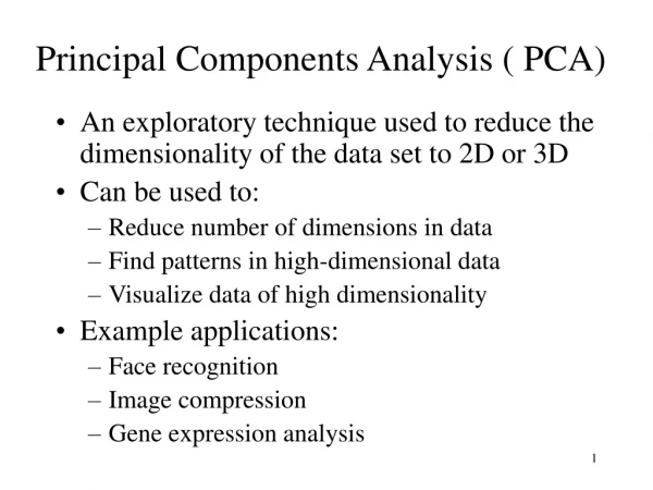
Overview: • What is Principal Component Analysis • Computing the compnents in PCA • Dimensionality Reduction using PCA • A 2D example in PCA • Applications of PCA in computer vision • Importance of PCA in analysing data in higher dimensions • Questions
Principal Component Analysis • Most common form of factor analysis • The new variables/dimensions – Are linear combinations of the original ones – Are uncorrelated with one another • Orthogonal in original dimension space – Capture as much of the original variance in the data as possible – Are called Principal Components
What are the new axes? • Orthogonal directions of greatest variance in data • Projections along PC1 discriminate the data most along any one axis
Principal Components • First principal component is the direction of greatest variability (covariance) in the data • Second is the next orthogonal (uncorrelated) direction of greatest variability – So first remove all the variability along the first component, and then find the next direction of greatest variability • And so on …
Principal Components Analysis (PCA) • Principle – Linear projection method to reduce the number of parameters – Transfer a set of correlated variables into a new set of uncorrelated variables – Map the data into a space of lower dimensionality – Form of unsupervised learning • Properties – It can be viewed as a rotation of the existing axes to new positions in the space defined by original variables – New axes are orthogonal and represent the directions with maximum variability
Computing the Components •Data points are vectors in a multidimensional space • Projection of vector x onto an axis (dimension) u is u.x • Direction of greatest variability is that in which the average square of the projection is greatest – I.e. u such that E((u.x)2) over all x is maximized – (we subtract the mean along each dimension, and center the original axis system at the centroid of all data points, for simplicity) – This direction of u is the direction of the first Principal Component
Computing the Components • E((u.x)2) = E ((u.x) (u.x)T) = E (u.x.xT.uT) • The matrix S = x.xT contains the correlations (similarities) of the original axes based on how the data values project onto them • So we are looking for w that maximizes uSuT, subject to u being unit-length • It is maximized when w is the principal eigenvector of the matrix S, in which case – uCuT = uλuT = λ if u is unit-length, where λ is the principal eigenvalue of the correlation matrix C – The eigenvalue denotes the amount of variability captured along that dimension
Why the Eigenvectors? MaximiseuTxxTus.t uTu= 1 Construct LangrangianuTxxTu– λuTu Vector of partial derivatives set to zero xxTu– λu = (xxT – λI) u = 0 As u ≠ 0 then u must be an eigenvector of xxT with eigenvalue λ
Computing the Components • Similarly for the next axis, etc. • So, the new axes are the eigenvectors of the matrix of correlations of the original variables, which captures the similarities of the original variables based on how data samples project to them • Geometrically: centering followed by rotation • – Linear transformation
PCs, Variance and Least-Squares • The first PC retains the greatest amount of variation in the sample • The kth PC retains the kth greatest fraction of the variation in the sample • The kth largest eigenvalue of the correlation matrix C is the variance in the sample along the kthPC • The least-squares view: PCs are a series of linear least squares fits to a sample, each orthogonal to all previous ones
How Many PCs? • For n original dimensions, correlation matrix is nxn, and has up to n eigenvectors. So n PCs. • Where does dimensionality reduction come from?
Dimensionality Reduction Can ignore the components of lesser significance. You do lose some information, but if the eigenvalues are small, you don’t lose much – n dimensions in original data – calculate n eigenvectors and eigenvalues – choose only the first p eigenvectors, based on their eigenvalues – final data set has only p dimensions
PCA Example –STEP 1 • Subtract the mean from each of the data dimensions. All the x values have x subtracted and y values have y subtracted from them. This produces a data set whose mean is zero. Subtracting the mean makes variance and covariance calculation easier by simplifying their equations. The variance and co-variance values are not affected by the mean value.
PCA Example –STEP 1 http://kybele.psych.cornell.edu/~edelman/Psych-465-Spring-2003/PCA-tutorial.pdf DATA: x y 2.5 2.4 0.5 0.7 2.2 2.9 1.9 2.2 3.1 3.0 2.3 2.7 2 1.6 1 1.1 1.5 1.6 1.1 0.9 ZERO MEAN DATA: x y .69 .49 -1.31 -1.21 .39 .99 .09 .29 1.29 1.09 .49 .79 .19 -.31 -.81 -.81 -.31 -.31 -.71 -1.01
PCA Example –STEP 1 http://kybele.psych.cornell.edu/~edelman/Psych-465-Spring-2003/PCA-tutorial.pdf
PCA Example –STEP 2 • Calculate the covariance matrix cov = .616555556 .615444444 .615444444 .716555556 • since the non-diagonal elements in this covariance matrix are positive, we should expect that both the x and y variable increase together.
PCA Example –STEP 3 • Calculate the eigenvectors and eigenvalues of the covariance matrix eigenvalues = .0490833989 1.28402771 eigenvectors = -.735178656 -.677873399 .677873399 -.735178656
PCA Example –STEP 3 http://kybele.psych.cornell.edu/~edelman/Psych-465-Spring-2003/PCA-tutorial.pdf • eigenvectors are plotted as diagonal dotted lines on the plot. • Note they are perpendicular to each other. • Note one of the eigenvectors goes through the middle of the points, like drawing a line of best fit. • The second eigenvector gives us the other, less important, pattern in the data, that all the points follow the main line, but are off to the side of the main line by some amount.
PCA Example –STEP 4 • Reduce dimensionality and form feature vector the eigenvector with the highest eigenvalue is the principle component of the data set. In our example, the eigenvector with the larges eigenvalue was the one that pointed down the middle of the data. Once eigenvectors are found from the covariance matrix, the next step is to order them by eigenvalue, highest to lowest. This gives you the components in order of significance.
PCA Example –STEP 4 Now, if you like, you can decide to ignore the components of lesser significance. You do lose some information, but if the eigenvalues are small, you don’t lose much • n dimensions in your data • calculate n eigenvectors and eigenvalues • choose only the first p eigenvectors • final data set has only p dimensions.
PCA Example –STEP 4 • Feature Vector FeatureVector = (eig1 eig2 eig3 … eign) We can either form a feature vector with both of the eigenvectors: -.677873399 -.735178656 -.735178656 .677873399 or, we can choose to leave out the smaller, less significant component and only have a single column: - .677873399 - .735178656
PCA Example –STEP 5 • Deriving the new data FinalData = RowFeatureVector x RowZeroMeanData RowFeatureVector is the matrix with the eigenvectors in the columns transposed so that the eigenvectors are now in the rows, with the most significant eigenvector at the top RowZeroMeanData is the mean-adjusted data transposed, ie. the data items are in each column, with each row holding a separate dimension.
PCA Example –STEP 5 FinalData transpose: dimensions along columns x y -.827970186 -.175115307 1.77758033 .142857227 -.992197494 .384374989 -.274210416 .130417207 -1.67580142 -.209498461 -.912949103 .175282444 .0991094375 -.349824698 1.14457216 .0464172582 .438046137 .0177646297 1.22382056 -.162675287
PCA Example –STEP 5 http://kybele.psych.cornell.edu/~edelman/Psych-465-Spring-2003/PCA-tutorial.pdf
Reconstruction of original Data • If we reduced the dimensionality, obviously, when reconstructing the data we would lose those dimensions we chose to discard. In our example let us assume that we considered only the x dimension…
Reconstruction of original Data http://kybele.psych.cornell.edu/~edelman/Psych-465-Spring-2003/PCA-tutorial.pdf x -.827970186 1.77758033 -.992197494 -.274210416 -1.67580142 -.912949103 .0991094375 1.14457216 .438046137 1.22382056
Applications in computer vision- PCA to find patterns- • 20 face images: NxN size • One image represented as follows- • Putting all 20 images in 1 big matrix as follows- • Performing PCA to find patterns in the face images • Idenifying faces by measuring differences along the new axes (PCs)
PCA for image compression: • Compile a dataset of 20 images • Build the covariance matrix of 20 dimensions • Compute the eigenvectors and eigenvalues • Based on the eigenvalues, 5 dimensions can be left out, those with the least eigenvalues. • 1/4th of the space is saved.
Importance of PCA • In data of high dimensions, where graphical representation is difficult, PCA is a powerful tool for analysing data and finding patterns in it. • Data compression is possible using PCA • The most efficient expression of data is by the use of perpendicular components, as done in PCA.
Questions: • What do the eigenvectors of the covariance matrix while computing the principal components give us? • At what point in the PCA process can we decide to compress the data? • Why are the principal components orthogonal? • How many different covariance values can you calculate for an n-dimensional data set?