Download
1 / 30
340 likes | 595 Views
Business Statistics in Practice. Chapter 11 Simple Linear Regression Analysis ( 线性回归分析 ). Two quantitative variables Correlation. A relationship between two variables. Explanatory (Independent)Variable. Response (Dependent)Variable. y. x. Hours of Training. Number of Accidents.

E N D
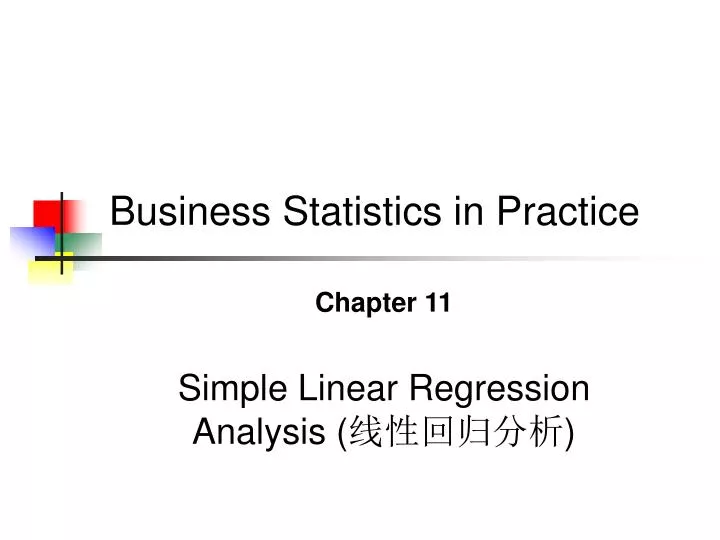
Business Statistics in Practice Chapter 11 Simple Linear Regression Analysis (线性回归分析)
Two quantitative variablesCorrelation A relationship between two variables. Explanatory (Independent)Variable Response (Dependent)Variable y x Hours of Training Number of Accidents Shoe Size Height Cigarettes smoked per day Lung Capacity Score on SAT Grade Point Average Height IQ What type of relationship exists between the two variables and is the correlation significant?
Correlation(相关) vs. Regression(回归) • A scatter diagram(散点图) can be used to show the relationship between two variables • Correlation (相关) analysis is used to measure strength of the association (linear relationship) between two variables • Correlation is only concerned with strength of the relationship • No causal effect (因果效应) is implied with correlation
Example The twelve days of stock prices and the overall market index on each day are given as follows: Price Index (000s) 8.0 7.5 7.5 7.3 7.2 7.2 7.1 7.1 7.0 6.2 6.2 5.1 96 92 91 88 86 85 84 83 82 79 78 69
The Coefficient of Correlation (r). It is a measure of the strength of the relationship (linear)between two variables It can range from -1.00 to 1.00.
The Coefficient of Correlation (r). Values of -1.00 or 1.00 indicate perfect and strong correlation. Negative values indicate an inverse relationship and positive values indicate a direct relationship. Values close to 0.0 indicate weak correlation.
Introduction to Regression Analysis • Regression analysis is used to: • Predict the value of a dependent variable based on the value of at least one independent variable • Explain the impact of changes in an independent variable on the dependent variable Dependent variable: the variable we wish to predict or explain Independent variable: the variable used to explain the dependent variable
Simple Linear Regression Model • Only one independent variable, X • Relationship between X and Y is described by a linear function • Changes in Y are assumed to be caused by changes in X
Types of Relationships Linear relationships Curvilinear relationships Y Y X X Y Y X X
Types of Relationships (continued) Strong relationships Weak relationships Y Y X X Y Y X X
Types of Relationships (continued) No relationship Y X Y X
Simple Linear Regression Model Random Error term Population SlopeCoefficient Population Y intercept Independent Variable Dependent Variable Linear component Random Error component
Simple Linear Regression Model (continued) Y Observed Value of Y for Xi εi Slope = β1 Predicted Value of Y for Xi Random Error for this Xi value Intercept = β0 X Xi
Simple Linear Regression Equation (Prediction Line) The simple linear regression equation provides an estimate of the population regression line Estimated (or predicted) Y value for observation i Estimate of the regression intercept Estimate of the regression slope Value of X for observation i The individual random error terms ei have a mean of zero
Least Squares Method (最小二乘方法) • b0 and b1 are obtained by finding the values of b0 and b1 that minimize the sum of the squared differences between Y and :
Interpretation of the Slope(斜率) and the Intercept(截距) • b0 is the estimated average value of Y when the value of X is zero • b1 is the estimated change in the average value of Y as a result of a one-unit change in X
The Least Square Point Estimates Least squares point estimate of the y-intercept 0
The House Price Case Example 11.1 • A real estate agent wishes to examine the relationship between the selling price of a home and its size (measured in square feet) • A random sample of 10 houses is selected • Dependent variable (Y) = house price in $1000s • Independent variable (X) = square feet
Graphical Presentation • House price model: scatter plot
Graphical Presentation • House price model: scatter plot and regression line Slope = 0.10977 Intercept = 98.248
Interpretation of the Intercept, b0 • b0 is the estimated average value of Y when the value of X is zero (if X = 0 is in the range of observed X values) • Here, no houses had 0 square feet, so b0 = 98.24833 just indicates that, for houses within the range of sizes observed, $98,248.33 is the portion of the house price not explained by square feet
Interpretation of the Slope Coefficient, b1 • b1 measures the estimated change in the average value of Y as a result of a one-unit change in X • Here, b1 = .10977 tells us that the average value of a house increases by .10977($1000) = $109.77, on average, for each additional one square foot of size
Predictions using Regression Analysis Predict the price for a house with 2000 square feet: The predicted price for a house with 2000 square feet is 317.85($1,000s) = $317,850
Model Assumptions • Mean of ZeroAt any given value of x, the population of potential error term values has a mean equal to zero • Constant Variance AssumptionAt any given value of x, the population of potential error term values has a variance that does not depend on the value of x • Normality AssumptionAt any given value of x, the population of potential error term values has a normal distribution • Independence AssumptionAny one value of the error term e is statistically independent of any other value of e
Example 11.2: Excel Output of Regression on Fuel Consumption Data
What Does r2 Mean? The coefficient of determination, r2, is the proportion of the total variation in the n observed values of the dependent variable that is explained by the simple linear regression model
Mechanics of the F Test • T test: To test H0: β1= 0 versus Ha: β1 0 at the a level of significance • Test statistics based on F • Reject H0 if F(model) > Fa or p-value < a • Fa is based on 1 numerator and n-2 denominator degrees of freedom
Chapter Summary • Discussed correlation -- measuring the strength of the association • Introduced types of regression models • Reviewed assumptions of regression and correlation • Discussed determining the simple linear regression equation • Addressed prediction of individual values • Model diagnostic